Download
1 / 18
180 likes | 303 Views
Forest response to cloud and canopy effects on incident radiation (& some other stuff). David R. Fitzjarrald Atmospheric Sciences Research Center University at Albany, SUNY with collaborators at ASRC (Staebler, Sakai,Czikowsky) & Geoffrey G. Parker

E N D
Forest response to cloud and canopy effects on incident radiation (& some other stuff) David R. Fitzjarrald Atmospheric Sciences Research Center University at Albany, SUNY with collaborators at ASRC (Staebler, Sakai,Czikowsky) & Geoffrey G. Parker Smithsonian Environmental Research Center
The great lubricated debate at Wascesiu Lake Saskatchwan, 1993 Resolved: The English system of units is superior to the Metric System The fervor of the recently converted vs. bullheadedness of a southern neighbor “What is your body volume in English units?” --Andy Black “If God wanted Canadians to use km, he wouldn’t have designed the Alberta road grid in miles!” --Old Gringo (“A pint’s a pound the world around”, but only in USA)
Is there role for eddy flux scientists once the measurement has been ‘tamed’? Raw data --> Terraflux imperial processing --> uniform time series gaps filled! wild points jettisoned! no surprises! modeler’s dream! ‘Good’ & ‘bad’ data bundled! It’s a mess! Large data storage requirement Labor intensive Still room for alternate ways to define the ensemble in Reynolds average (thinking of HaPe’s talk yesterday--think about ‘event-based’ composites) Defining the ensemble average: • time average (conventional, many techniques to use) • spatial average (remote sensors) • average of repeated realizations
December 8, 2001 Ceilometer Backscatter Profile Cloud base PAR down Sdown 1:30 PM LT 3:00 PM LT 4:30 PM LT Rain No precip. recorded by the rain gauge in this event!
We estimated rainfall interception using eddy flux data. Czikowsky & Fitzjarrald, 2009. J. Hydrology 377 92-105. Find enough data with ‘similar’ conditions. t = 0 defined by a clear ‘event’ : event based composite for ensemble mean
Old way: Describe vegetation responses to to the imposed environment. • How does vegetation define its own local environment? • Do natural ‘clocks’ overrule immediate influence of local environment? (do we really desperately need continuous time series of 1/2 hour fluxes?) • A first step: how to describe fine scale microclimatic temporal changes Wind abstract information to u* fluctuating <- time response input: Sdn (clouds, aerosols) ; stomatal response Light larger time scales diurnal variation <- circadian rhythms annual --> phenological effects steady <- photoinhibition <- direct vs. diffuse radiation Temperature following light, with cp, storage ∂/∂t modulation
Doughty, C. E., and M. L. Goulden (2008), Are tropical forests near a high temperature threshold? J. Geophys. Res., 113, G00B07 Tleaf Tcanopy gs-branch PARdn Gc H, LE FCO2 Rnet, sum
Cloudy days with higher uptake occur in regular sequence (HF) Freedman & Fitzjarrald (2000)
Study area location Amazon R. Tapajos R. Km 67 : LBA Old-growth rain forest site(Lat: 2.88528 S ; Lon:54.92047 W)
km67 site 1) Eddy covariance system at ~ 60 m (Harvard U), including: Campbell CSAT 3-D Sonic Anemometer Licor 6262 CO2/H2O analyzer 2) Precipitation gauge at 42 m height (1-minute data) 3) Vaisala CT-25K Ceilometer operating during periods from April 2001 to July 2003 (30-m resolution backscatter profile every 15 seconds) Ceilometer 4) Radiation boom at 60 m (Lup, Ldn, Sup, Sdown, PARup PARdn) 5) Temperature, RH profile
Little variation in day-to-day cloud fraction and cloud base during the dry season
subcanopy radiation array 1 1 15 16 11 14 4 meters Sdn but with colocated PAR at station 1
Analysis in progress: ‘conventional’ use of the light data already done by Jess Parker at SERC
incident at the subcanopy penetrance reflectance brightness classes 1 (<30%), 2 (30-60%), 3 (60-90%), and 4 (>90%) - % incoming light relative to modeled clear conditions. penetrance to the understory and reflectance from the top. (half-hour averages of calibrated array means) source: Parker, Fitzjarrald, and Sampaio, LBA Symposium poster, 2006.
next steps: • Identify dark-to-light transitions objectively: defines t = 0 • construct longitudinal ensemble averages • find the perturbation w’ and CO2’ for a large number of realizations • generate Fco2 as function of the light ‘jump’, background microenvironment from LBA-ECO Tapajós 2003 from N-OJP BOREAS 1994
The “Cloud of Turin” 8/8/1988 Kuskokwim River delta, Alaska.