Download
1 / 114
1.18k likes | 1.52k Views
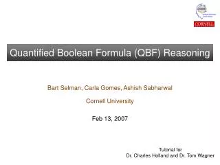
Quantified Boolean Formula (QBF) Reasoning. Bart Selman, Carla Gomes, Ashish Sabharwal Cornell University Feb 13, 2007. Tutorial for Dr. Charles Holland and Dr. Tom Wagner. Tutorial Roadmap. Automated reasoning The complexity challenge State of the art in Boolean reasoning

E N D
Quantified Boolean Formula (QBF) Reasoning Bart Selman, Carla Gomes, Ashish Sabharwal Cornell University Feb 13, 2007 Tutorial forDr. Charles Holland and Dr. Tom Wagner
Tutorial Roadmap • Automated reasoning • The complexity challenge • State of the art in Boolean reasoning • SAT-based reasoning • Boolean logic • Search space, worst-case complexity • Hardness profiles, scaling in practice • Modeling problems as SAT • Example domain: planning • QBF reasoning (extends SAT) • A new range of applications • Two motivating examples • network planning, logistics planning • Quantified Boolean logic • Modeling problems as QBF • Search space, worst-case complexity • Scaling in practice • High-Performance QBF reasoning • Key research advances • The technology behind QBF • A. New modeling techniques • B. Learning while reasoning • C. Structure discovery • Experimental Results • Summary
Tutorial Roadmap • Automated reasoning • The complexity challenge • State of the art in Boolean reasoning • SAT-based reasoning • Boolean logic • Search space, worst-case complexity • Hardness profiles, scaling in practice • Modeling problems as SAT • Example domain: planning • QBF reasoning (extends SAT) • A new range of applications • Two motivating examples • network planning, logistics planning • Quantified Boolean logic • Modeling problems as QBF • Search space, worst-case complexity • Scaling in practice • High-Performance QBF reasoning • Key research advances • The technology behind QBF • A. New modeling techniques • B. Learning while reasoning • C. Structure discovery • Experimental Results • Summary
The Quest for Machine Reasoning Objective: Develop foundations and technology to enable effective, practical, large-scale automated reasoning. Machine Reasoning (1960-90s) Current reasoning technology Computational complexityof reasoning appearsto severely limit real-world applications Revisiting the challenge: Significant progress with new ideas / tools for dealing with complexity (scale-up), uncertainty, and multi-agent reasoning
General Automated Reasoning GeneralInferenceEngine ModelGenerator(Encoder) Probleminstance Solution Domain-specific Generic e.g. logistics, war games,chess, space missions, planning, scheduling, ... applicable to all domainswithin range of modeling language Research objective Better reasoning and modeling technology Impact Faster solutions in several domains
Simple Example: Knowledge Base Variables (binary) X1 = email_ received X2 = in_ meeting X3 = urgent X4 = respond_to_email X5 = near_deadline X6 = postpone X7 = air_ticket_info_request X8 = travel_ request X9 = info_request • Rules: • X1 & (not X2) & X3 X4 • X2 not X4 • X5 X3 or X6 • 4. X7 X8 • 5. X8 X9 • 6. X8 X5 • 7. X6 not X9 Question: Given: X1= true; X2 = false; X7=true. What is X4 = ? Answer Development: Inference Chain Step 1: X7 X8 (rule 4) Step 2: X8 X5 (rule 6) Step 3: X5 X3 or X6 (rule 3) M Case A: X6 = true Step 4: X6 not X9 Step 5: X9 not X8 Step 6: Contradiction Backtrack to M Case B: X3 = true X1 & (not X2) & X3 X4 Step 7: X4 = true (Rule 1) Reasoning Complexity • EXPONENTIAL COMPLEXITY: INHERENT • ANworst case • N= No. of Variables/Objects A= Object states • TIME/SPACE • Granularity Object states • Current implementations trade • time with soundness Search for rules to apply For N variables: 2N cases drive complexity! Check Contradictions
Complexity Exponential Exponential Complexity Growth: The Challenge of Complex Domains Note: rough estimates, for propositional reasoning 1M 5M War Gaming 10301,020 0.5M 1M VLSI Verification 10150,500 Case complexity 100K 450K Military Logistics 106020 20K 100K Chess (20 steps deep) 103010 No. of atoms on the earth 10K 50K Deep space mission control Seconds until heat death of sun 1047 100 200 1030 Car repair diagnosis Protein folding Calculation (petaflop-year) Variables 100 10K 20K 100K 1M Rules (Constraints) [Credit: Kumar, DARPA; Cited in Computer World magazine]
Tutorial Roadmap • Automated reasoning • The complexity challenge • State of the art in Boolean reasoning • SAT-based reasoning • Boolean logic • Search space, worst-case complexity • Hardness profiles, scaling in practice • Modeling problems as SAT • Example domain: planning • QBF reasoning (extends SAT) • A new range of applications • Two motivating examples • network planning, logistics planning • Quantified Boolean logic • Modeling problems as QBF • Search space, worst-case complexity • Scaling in practice • High-Performance QBF reasoning • Key research advances • The technology behind QBF • A. New modeling techniques • B. Learning while reasoning • C. Structure discovery • Experimental Results • Summary
Progress in Last 15 Years Focus: Combinatorial Search Spaces Specifically, the Boolean satisfiability problem, SAT Significant progress since the 1990’s. How much? • Problem size: We went from 100 variables, 200 constraints (early 90’s) to 1,000,000 vars. and 5,000,000 constraints in 15 years.Search space: from 10^15 to 10^300,000.[Aside: “one can encode quite a bit in 1M variables.”] • Tools: 50+ competitive SAT solvers available Overview of state of the art: Plenary talk at IJCAI-05 (Selman); Gomes and Selman, Nature ’05
How Large are the Problems? A bounded model checking problem:
SAT Encoding (automatically generated from problem specification) i.e., ((not x1) or x7) ((not x1) or x6) etc. x1, x2, x3, etc. are our Boolean variables (to be set to True or False) Should x1 be set to False??
10 Pages Later: … i.e., (x177 or x169 or x161 or x153 … x33 or x25 or x17 or x9 or x1 or (not x185)) clauses / constraints are getting more interesting… Note x1 …
Finally, 15,000 Pages Later: Search space of truth assignments: Current SAT solvers solve this instance in under 30 seconds!
SAT Solver Progress Solvers have continually improved over time Source: Marques-Silva 2002
How do SAT Solvers Keep Improving? From academically interesting to practically relevant. We now have regular SAT solver competitions. (Germany ’89, Dimacs ’93, China ’96, SAT-02, SAT-03, SAT-04, SAT-05, SAT-06) E.g. at SAT-2006 (Seattle, Aug ’06): • 35+ solvers submitted, most of them open source • 500+ industrial benchmarks • 50,000+ benchmark instances available on the www This constant improvement in SAT solvers is the key to making, e.g.,SAT-based planning very successful.
Current Automated Reasoning Tools Most-successful fully automated methods: based on Boolean Satisfiability (SAT) / Propositional Reasoning • Problems modeled as rules / constraints over Boolean variables • “SAT solver” used as the inference engine Applications: single-agent search • AI planning SATPLAN-06, fastest optimal planner; ICAPS-06 competition (Kautz & Selman ’06) • Verification – hardware and software Major groups at Intel, IBM, Microsoft, and universitiessuch as CMU, Cornell, and Princeton.SAT has become the dominant technology. • Many other domains: Test pattern generation, Scheduling,Optimal Control, Protocol Design, Routers, Multi-agent systems,E-Commerce (E-auctions and electronic trading agents), etc.
Tutorial Roadmap • Automated reasoning • The complexity challenge • State of the art in Boolean reasoning • SAT-based reasoning • Boolean logic • Search space, worst-case complexity • Hardness profiles, scaling in practice • Modeling problems as SAT • Example domain: planning • QBF reasoning (extends SAT) • A new range of applications • Two motivating examples • network planning, logistics planning • Quantified Boolean logic • Modeling problems as QBF • Search space, worst-case complexity • Scaling in practice • High-Performance QBF reasoning • Key research advances • The technology behind QBF • A. New modeling techniques • B. Learning while reasoning • C. Structure discovery • Experimental Results • Summary
Boolean Logic Defined over Boolean (binary) variablesa, b, c, … Each of these can be True (1) or False (0) Variables connected together with logic operators: and, or, not (denoted ) E.g. (a or b) is True iff at least one of a and b is True ((c and d)) or f) is True iff either c is True and d is False, or f is True Fact: All other Boolean logic operators can be expressed with and, or, not E.g. (a b) same as (a or b) Boolean formula, e.g. F = (a or b) and (a and (b or c)) (Truth) Assignment: any setting of the variables to True or False Satisfying assignment: assignment where the formula evaluates to True
Boolean Logic: Example F = (a or b) and (a and (b or c)) Note: True often written as 1, False as 0 • There are 23 = 8 possible truth assignments to a, b, c • (a=0,b=1,c=0) representing (a=False, b=True, c=False) • (a=0,b=0,c=1) • … • Exactly 3 truth assignments satisfy F • (a=0,b=1,c=0) • (a=0,b=1,c=1) • (a=1,b=0,c=0)
Boolean Logic: Expressivity All discrete single-agent search problems can be cast as a Boolean formula! Variables a, b, c, … often represent “states” of the system, “events”, “actions”, etc. (more on this later, using Planning as a example) Very general encoding language. E.g. can handle • Numbers (k-bit binary representation) • Floating-point numbers • Arithmetic operators like +, x, exp(), log() • … SAT encodings (generated automatically from high level languages) routinely used in domains like planning, scheduling, verification, e-commerce, network design, … Recall Example: “event” Variables X1 = email_ received X2 = in_ meeting X3 = urgent X4 = respond_to_email X5 = near_deadline X6 = postpone X7 = air_ticket_info_request X8 = travel_ request X9 = info_request “state” “action” • Rules: • X1 & (not X2) & X3 X4 • X2 not X4 • X5 X3 or X6 • 4. X7 X8 • 5. X8 X9 • 6. X8 X5 • 7. X6 not X9 constraint
Boolean Logic: Standard Representations Each problem constraint typically specified as (a set of) clauses: E.g. (a or b), (c or d or f), (a or c or d), … Formula in conjunctive normal form, or CNF: a conjunction of clauses E.g. F = (a or b) and (a and (b or c)) changes to FCNF = (a or b) and (a or b) and (b or c) Alternative [useful for QBF]: specify each constraint as a term(only “and”, “not”): E.g. (a and d), (b and a and f), (b and d and e), … Formula in disjunctive normal form, or DNF: a disjunction of terms E.g. FDNF = (a and b) or (a and b and c) clauses (only “or”, “not”)
Boolean Satisfiability Testing • A wide range of applications • Relatively easy to test for small formulas (e.g. with a Truth Table) • However, very quickly becomes hard to solve • Search space grows exponentially with formula size(more on this next) SAT technology has been very successful in taming this exponential blow up! • The Boolean Satisfiability Problem, or SAT: • Given a Boolean formula F, • find a satisfying assignment for F • or prove that no such assignment exists.
Tutorial Roadmap • Automated reasoning • The complexity challenge • State of the art in Boolean reasoning • SAT-based reasoning • Boolean logic • Search space, worst-case complexity • Hardness profiles, scaling in practice • Modeling problems as SAT • Example domain: planning • QBF reasoning (extends SAT) • A new range of applications • Two motivating examples • network planning, logistics planning • Quantified Boolean logic • Modeling problems as QBF • Search space, worst-case complexity • Scaling in practice • High-Performance QBF reasoning • Key research advances • The technology behind QBF • A. New modeling techniques • B. Learning while reasoning • C. Structure discovery • Experimental Results • Summary
Fix one variable to True or False Fix another var Fix a 3rd var Fix a 4th var True False False True False SAT Search Space All vars free SAT Problem: Find a path to a True leaf node. For N Boolean variables, the raw search space is of size 2N • Grows very quickly with N • Brute-force exhaustive search unrealistic without efficient heuristics, etc.
exponential polynomial Worst-Case Complexity SAT is an NP-complete problem • Worst-case believed to be exponential(roughly 2N for N variables) • 10,000+ problems in CS are NP-complete (e.g. planning, scheduling, protein folding, reasoning) • P vs. NP --- $1M Clay Prize However, real-world instances are usually not pathological and can often be solved very quickly with the latest technology! Typical-case complexity provides a moredetailed understanding and a more positive picture.
Tutorial Roadmap • Automated reasoning • The complexity challenge • State of the art in Boolean reasoning • SAT-based reasoning • Boolean logic • Search space, worst-case complexity • Hardness profiles, scaling in practice • Modeling problems as SAT • Example domain: planning • QBF reasoning (extends SAT) • A new range of applications • Two motivating examples • network planning, logistics planning • Quantified Boolean logic • Modeling problems as QBF • Search space, worst-case complexity • Scaling in practice • High-Performance QBF reasoning • Key research advances • The technology behind QBF • A. New modeling techniques • B. Learning while reasoning • C. Structure discovery • Experimental Results • Summary
Delete Constraints Add Constraints Typical-Case Complexity A key hardness parameter for k-SAT: the ratio of clauses to variables Problems that are not critically constrained tend to be much easier in practicethan the relatively few critically constrained ones [Mitchell, Selman, and Levesque ’92; Kirkpatrick and Selman – Science ’94]
Phase transition Random 3-SAT as of 2004 Linear time algs. Random Walk DP DP’ GSAT Walksat SP Typical-Case Complexity SAT solvers continually getting close to tackling problems in the hardest region! SP (survey propagation) now handles 1,000,000 variablesvery near the phase transition region
Tractable Sub-Structure Can Dominate and Drastically Reduce Solution Cost! 2+p-SAT model: mix 2-SAT (tractable) and 3-SAT (intractable) clauses > 40% 3-SAT: exponential scaling Median runtime 40% 3-SAT: linear scaling! Number of variables (Monasson, Selman et al. – Nature ’99; Achlioptas ’00)
Tutorial Roadmap • Automated reasoning • The complexity challenge • State of the art in Boolean reasoning • SAT-based reasoning • Boolean logic • Search space, worst-case complexity • Hardness profiles, scaling in practice • Modeling problems as SAT • Example domain: planning • QBF reasoning (extends SAT) • A new range of applications • Two motivating examples • network planning, logistics planning • Quantified Boolean logic • Modeling problems as QBF • Search space, worst-case complexity • Scaling in practice • High-Performance QBF reasoning • Key research advances • The technology behind QBF • A. New modeling techniques • B. Learning while reasoning • C. Structure discovery • Experimental Results • Summary
SAT Encoding Example: Planning Domain Planning Problem Propositional CNF formulaby axiom schemas Discrete time, modeled by integers • state predicates: indexed by time at which they hold E.g. at_location(x,,loc,i), free(x,i+1), route(cityA,cityB,i) • action predicates: indexed by time at which action begins E.g. fly(cityA,cityB,i), pickup(x,loc,i), drive_truck(loc1,loc2,i) • each action takes 1 time step • many actions may occur at the same step
Encoding Rules • Actions imply preconditions and effects fly(x,y,i) at(x,i) and route(x,y,i) and at(y,i+1) • Conflicting actions cannot occur at same time (A deletes a precondition of B) fly(x,y,i) and yz not fly(x,z,i) • If something changes, an action must have caused it(Explanatory Frame Axioms) at(x,i) and not at(x,i+1) y . route(x,y) and fly(x,y,i) • Initial and final states hold at(NY,0) and ... and at(LA,9) and ...
Using SAT Solvers for Planning Modeling and Solving a Planning Problem instantiated propositional clauses instantiate Problem description inhigh level language axiom schemas (manual) length mapping SAT engine(s) interpret satisfying model plan (fully automatic)
Planning Benchmark Complexity Logistics domain – a complex, highly-parallel transportation domain E.g. logistics.d problem: • 2,165 possible actions per time slot • optimal solution contains 74 distinct actions over 14 time slots (out of 5 x 10^46 possible sequential plans of length 14) Satplan [Selman et al.] approach is currently fastest optimal planning approach. Winner ICAPS-05 & ICAPS-06 international planning competitions.
Tutorial Roadmap • Automated reasoning • The complexity challenge • State of the art in Boolean reasoning • SAT-based reasoning • Boolean logic • Search space, worst-case complexity • Hardness profiles, scaling in practice • Modeling problems as SAT • Example domain: planning • QBF reasoning (extends SAT) • A new range of applications • Two motivating examples • network planning, logistics planning • Quantified Boolean logic • Modeling problems as QBF • Search space, worst-case complexity • Scaling in practice • High-Performance QBF reasoning • Key research advances • The technology behind QBF • A. New modeling techniques • B. Learning while reasoning • C. Structure discovery • Experimental Results • Summary
The Next Challenge in Reasoning Technology Multi-Agent Reasoning:Quantified Boolean Formulae (QBF) • Allow use of Forall and Exists quantifiers over Boolean variables • QBF significantly more expressive than SAT: from single-person puzzles to competitive games! New application domains: • Unbounded length planning and verification • Multi-agent scenarios, strategic decision making • Adversarial settings, contingency situations • Incomplete / probabilistic information But, computationally *much* harder (formally PSPACE-complete rather than NP-complete) war gaming Key challenge: Can we do for QBF what was done for SAT solving in the last decade? Would open up a tremendous range of advanced automated reasoning capabilities!
Multi-Agent Reasoning A Wide Range of Applications • Logistics planning and scheduling under adversarial / uncertain conditions • Multi-agent contingency planning with performance guarantees • Analysis and validation of distributed agent strategies and coordination • Event logic • Reasoning in rich multi-player (adversarial) settings • War gaming, designing secure data and communication networks QBF Technology for Multi-Agent Reasoning offers: • Performance guarantee / optimality / “worst-case” scenario analysis • NOTE: Worst-case may be rare but can have catastrophic consequences! The Challenge: Overcoming the high computational complexity
SAT Reasoning vs. QBF Reasoning SAT Reasoning • Combinatorial search for optimal and near-optimal solutions • NP-complete(hard) • planning, scheduling, verification, model checking, … • From 200 vars in early ’90s to 1M vars. Now a commercially viable technology. QBF Reasoning • Combinatorial searchfor optimal and near-optimal solutions in multi-agent, uncertain, orhostile environments • PSPACE-complete(harder) • adversarial planning, gaming, security protocols, contingency planning, … • From 200 vars in late 90’s to 100K vars currently. Still rapidly moving. Scope oftechnology Worst-casecomplexity Applicationareas Researchstatus
Tutorial Roadmap • Automated reasoning • The complexity challenge • State of the art in Boolean reasoning • SAT-based reasoning • Boolean logic • Search space, worst-case complexity • Hardness profiles, scaling in practice • Modeling problems as SAT • Example domain: planning • QBF reasoning (extends SAT) • A new range of applications • Two motivating examples • network planning, logistics planning • Quantified Boolean logic • Modeling problems as QBF • Search space, worst-case complexity • Scaling in practice • High-Performance QBF reasoning • Key research advances • The technology behind QBF • A. New modeling techniques • B. Learning while reasoning • C. Structure discovery • Experimental Results • Summary
The Need for QBF Technology SAT technology, while very successful for single-agent search, is not suitable for adversarial reasoning. Must model the adversary and incorporate his actions into reasoning • SAT does not provide a framework for this • In fact, it cannot (more on this later) Two examples next: • Network planning: create a data/communication network between N nodes which is robust under failures during and after network creation • Logistics planning: achieve a transportation goal in uncertain environments
Adversarial Planning: Motivating Example Network Planning Problem: • Input: 5 nodes, 9 available edges that can be placed between any two nodes • Goal: all nodes finally connected to each other (directly or indirectly) • Requirement (A): final network must be robust against 2 node failures • Requirement (B): network creation process must be robust against 1 node failure E.g. a sample robust final configuration:(uses only 8 edges) • Side note: Mathematical structure of the problem: • (A) implies every node must have degree ≥ 3(otherwise it can easily be “isolated”) • At least one node must have degree ≥ 4(follows from 1. and that not all 5 nodes can have odd degree in any graph) • Need at least 8 edges total (follows from 1. and 2.) • If one node fails during creation, the remaining 4 must be connected with 6 edges to satisfy (A) • Actually need 9 edges to guarantee construction (follows from 4. because a node may fail as soon as its degree becomes 3)
Example: A SAT-Based Sequential Plan Ideal situation: No failure during network creation Create edge Next move if no failures Final network robust against2 failures The plan goes smoothly and we end up with the target network, which is robust against any 2 node failures
Example: A SAT-Based Sequential Plan Ideal situation: No failure during network creation Node failures may render the original plan ineffective, but re-planning could help makethe remaining network robust. What if the leftnode fails? Create edge Node failure during network creation Next move if a particular node fails • Can still make the remaining 4 nodesrobust using 2 more edges (total 8 used) • Feasible, but must re-planto find a different final configuration Next move if no failures Final network robust against2 more failures
Example: A SAT-Based Sequential Plan Ideal situation: No failure during network creation • Trouble! Can get stuck if • Resources are limited(only 9 edges) • Adversary is smart(takes out node with degree 4) • Poor decisions were made early on in the network plan What if the topnode fails? • Need to create 4 more edges tomake the remaining 4 nodes robust • Stuck! Have already used up 6 of the 9 available edges!
Example: A QBF-Based Contingency Plan • A QBF solver will return a robust contingency plan (a tree) • Will consider all relevant failure modes and responses • (only some “interesting” parts of the plan tree are shown here) …. …. …. …. …. …. …. …. …. …. only 8edgesused Create edge Node failure during network creation Next move if a particular node fails Next move if no failures 9 edgesneeded Final networks robust against2 more failures only 8edgesused 9 edgesneeded
Another Example: Logistics Planning (2) QbPlan (1) SatPlan • Blue nodes are cities, green nodes are military bases • Blue edges are commercial transports, green edges are military • Green edges (transports) have a capacity of 60 people, blue edges have a capacity of 100 people • operator: “transport” t(who, amount, from, to, step) • parallel actions can be taken at each step • Goal: Send 60 personal from Base-1 to Base-2 in at most 3 steps City-1 Base 2 *At any step commercial player can transport up to 80 civilians (s2) (s1) (s3) (s3) (s1) (s2) Base 1 City-2 City-4 20p 60p 20p 20p (s1) (s2) 60p (s1) (s2) City-3 (60p) + (80c) > 100 (civilian transport capacity) Re-planning needed !!! (20p) + (up to 80c) <= 100 • One player: military player, deterministic classic planning, SatPlan • (1) Sat-Plan: t(m, 60, base-1, city-3, 1), t(m, 60, city-3, city-4, 2), t(m, 60, city-4, base-2, 3) • Two players: deterministic adversarial planning QB Plan • Military Player (m) is “white player”, Commercial Player (c) is “black player” (Chess analogy). Commercial player can move up to 80 civilians between cities. Commercial moves can not be invalidated. Goal can be read as: “send 60 personal from Base-1 to Base-2 in at most 3 steps whatever commercial needs (moves) are” • If commercial player decides to move 80 civilians from city-3 to city-4 at the second step, we should replan (1). Indeed, the goal can not be achieved if we have already taken the first action of (1) • (2) QB-Plan: t(m, 20, base-1, city-1, 1), t(m, 20, base-1, city-2, 1), t(m, 20, base-1, city-3, 1), t(m, 20, city-1, city-4, 2), t(m, 20, city-2, city-4, 2), t(m, 20, city-3, city-4, 2), t(m, 60, city-4, base-2, 3)
Tutorial Roadmap • Automated reasoning • The complexity challenge • State of the art in Boolean reasoning • SAT-based reasoning • Boolean logic • Search space, worst-case complexity • Hardness profiles, scaling in practice • Modeling problems as SAT • Example domain: planning • QBF reasoning (extends SAT) • A new range of applications • Two motivating examples • network planning, logistics planning • Quantified Boolean logic • Modeling problems as QBF • Search space, worst-case complexity • Scaling in practice • High-Performance QBF reasoning • Key research advances • The technology behind QBF • A. New modeling techniques • B. Learning while reasoning • C. Structure discovery • Experimental Results • Summary
Quantified Boolean Logic Boolean logic extended with “quantifiers” on the variables • “there exists a value of x in {True,False}”, represented by x • “for every value of y in {True,False}”, represented by y • The rest of the Boolean formula structure similar to SAT,usually specified in CNF form E.g. QBF formula F(v,w,x,y) = vwxy : (v or w or x) and (v or w) and (v or y) Quantified Boolean variables constraints (as before)
Quantified Boolean Logic: Semantics F(v,w,x,y,z) = vwxy : (v or w or x) and (v or w) and (v or y) What does this QBF formula mean? Semantic interpretation: F is True iff “There exists a value of v s.t.for both values of wthere exists a value of x s.t.for both values of y(v or w or x) and (v or w) and (v or y) is True”