Download
1 / 33
330 likes | 473 Views
Beating Brute Force Search for QBF Satisfiability. Rahul Santhanam University of Edinburgh (joint work with Ryan Williams). Plan of the Talk. Introduction Background Results Algorithmic Results Small Number of Quantifier Alternations Large Number of Quantifier Alternations

E N D
Beating Brute Force Search for QBF Satisfiability RahulSanthanam University of Edinburgh (joint work with Ryan Williams)
Plan of the Talk • Introduction • Background • Results • Algorithmic Results • Small Number of Quantifier Alternations • Large Number of Quantifier Alternations • Implications for Circuit Complexity • Future Directions
Plan of the Talk • Introduction • Background • Results • Algorithmic Results • Small Number of Quantifier Alternations • Large Number of Quantifier Alternations • Implications for Circuit Complexity • Future Directions
The QBFSAT Problem • Input: A quantified Boolean formula ψ = Q1 X1 Q2 X2 ... QkXkφ(X1, ... , Xk) • Qi’s are quantifiers in {, } : if Qi = , then Qi+1 = , and conversely • Xi’s are blocks of variables • This is a k-QBFSAT instance. The number of alternationsis k-1 (alternatively, the number of quantifier blocks is k) • φ is by default a formula in CNF if Qk = , else in DNF (more generally, it could be a Boolean formula/circuit) • Question: Is ψ true?
The QBFSAT Problem x Ψ = x y z (x V y) Λ (x’ V z) y y z z z z 0 0 1 1 0 1 0 1
The QBFSAT Problem x Ψ = x y z (x V y) Λ (x’ V z) y y z z z z 0 0 1 1 0 1 0 1 Ψ is a YES instance
Easy Facts • Brute Force Search: QBFSAT can be solved in time 2n poly(m) on QBFs of size m with n variables • Hardness: QBFSAT is PSPACE-complete • QBFSAT is unlikely to be in P, but can we do better than brute-force search?
Conventional Algorithmic Paradigms for Satisfiability • DLL/Branching Algorithms: Explore tree of potential assignments by iteratively choosing variables to branch on • Local Search: Perform local search of solution space for a satisfying assignment
Conventional Algorithmic Paradigms applied to QBFSAT • DLL/Branching Algorithms: Power of DLL algorithms for SAT comes from choice of variables to branch on. For QBFs, this choice is much more restricted • Local Search: “Solutions” are not polynomial-size any more, so search of solution space becomes infeasible
Notation • Given a function s: N → N, we say that QBFSAT has savings s if there is an algorithm for QBFSAT running in time 2n-s(n) poly(m), where n is the number of variables and m the instance size • We call savings ω(log(n)) non-trivial • C-SAT:Satisfiability problem for circuit class C
The Relevance of Theory to Practice • Algorithmic ideas which make implementations more effective/efficient • Insights into the structure of hard instances
Plan of the Talk • Introduction • Background • Results • Algorithmic Results • Small Number of Quantifier Alternations • Large Number of Quantifier Alternations • Implications for Circuit Complexity • Future Directions
Our Results: Algorithms • Theorem 1: k-QBFSAT has savings Ω(n1/(k+1)) when m = poly(n) (Note that this is non-trivial when k = o(log(n)/loglog(n)) • Theorem 2: k-QBFSAT has savings Ω(k) (Note that this is non-trivial when k = ω(log(n)))
Our Results: Connections to Circuit Lower Bounds • Theorem 3: Non-trivial savings for QBFSAT would imply NEXP does not have poly-size Boolean formulas • Theorem 4: Savings Ω(nω(1)/k) for k-QBFSAT would imply NEXP does not have poly-size Boolean formulas
Plan of the Talk • Introduction • Background • Results • Algorithmic Results • Small Number of Quantifier Alternations • Large Number of Quantifier Alternations • Implications for Circuit Complexity • Future Directions
Reminder of Theorem 1 • Theorem 1: k-QBFSAT has savings Ω(n1/(k+1)) when m = poly(n)
Reminder of Theorem 1 • Theorem 1: k-QBFSAT has savings Ω(n1/(k+1)) when m = poly(n) • Proof Idea: Branching + memoization • Let ψ = Q X Q’ Y φ(X,Y), where |X| = n-n1/(k+1), and Q, Q’ are strings of quantifiers • Let f(X) = Q’ Y φ(X,Y). First compute the truth table of f in time O(2n-n^{1/(k+1)}) • To solve ψ, branch on X, using stored truth table to answer leaf queries in the branching tree. This can again be done in time O(2n-n^{1/(k+1)})
Plan of the Talk • Introduction • Background • Results • Algorithmic Results • Small Number of Quantifier Alternations • Large Number of Quantifier Alternations • Implications for Circuit Complexity • Future Directions
Proof Sketch for Theorem 2 • Reminder of Theorem 2: k-QBFSAT has savings Ω(k) • The algorithm works even when φ (the quantifier-free part) is a Boolean circuit • Somewhat counter-intuitive: Problem gets easier when number of alternations increases!
The Idea • Essentially same as “game tree evaluation” of [Snir85] and [Saks-Wigderson86] • Evaluate existential and universal branches randomly, halting the existential search when a 1 is returned and the universal search when a 0 is returned • In either the YES or NO case, this saves Ω(1) bits on average for every two consecutive alternations
Illustration x Ψ = x y z (x V y) Λ (x’ V z) Right branch, chosen with probability 1/2 y y z z z z 0 0 1 1 0 1 0 1 Ψ is a YES instance
Plan of the Talk • Introduction • Background • Results • Algorithmic Results • Small Number of Quantifier Alternations • Large Number of Quantifier Alternations • Implications for Circuit Complexity • Future Directions
Improved Algorithms? • Can we hope to achieve better savings than in Theorems 1 and 2? • How do different variants of QBFSAT relate to each other, eg., when φ is a Boolean formula as opposed to a CNF?
Reducing FormulaSAT to QBFSAT • Lemma 1: There is a polynomial-time algorithm which, given as input any Boolean formula on n variables of size poly(n), outputs an equivalent QBFSAT instance with n+O(log(n)) variables, size poly(n) and O(log(n)) alternations • Complexity inspiration: Classical result that NC1 = ALOGTIME • Much more efficient than Tseitin transformation
Reducing QBFormulaSAT to QBFSAT • Lemma 1’: There is a polynomial-time algorithm which, given as input any quantified Boolean formula with k’ alternations on n variables of size poly(n), outputs an equivalent QBFSAT instance with n+O(log(n)) variables, size poly(n) and k’+O(log(n)) alternations • Complexity inspiration: Classical result that NC1 = ALOGTIME
Implications • Corollary: If QBFSAT in time 1.9n, then QBFormulaSAT in time 1.9n+o(n) • By Williams’ algorithms-lbs connection for formulas, if FormulaSAT has savings ω(log(n)), then NEXP does not have poly-size formulas • Reminder of Theorem 4: Non-trivial savings for QBFSAT would imply NEXP does not have poly-size formulas • Proof: By Lemma 1, non-trivial savings for QBFSAT imply non-trivial savings for FormulaSAT
Reducing FormulaSAT to k-QBFSAT • Lemma 2: There is a polynomial-time algorithm which, given as input any Boolean formula on n variables of size poly(n), outputs an equivalent QBFSAT instance with n+O(n1/k) variables, size poly(n) and O(k) alternations • Complexity inspiration: Nepomnjascii’s result that every language in NC1 in Σk-LIN for some fixed k
Reducing QBFormulaSAT to k-QBFSAT • Lemma 2’: There is a polynomial-time algorithm which, given as input any quantified Boolean formula with k’ alternations on n variables of size poly(n), outputs an equivalent QBFSAT instance with n+O(n1/k) variables, size poly(n) and k’+O(k) alternations • Complexity inspiration: Nepomnjascii’s result that every language in NC1 in Σk-LIN for some fixed k
Implications • Corollary: If k-QBFSAT in time 1.9n, then QBFormulaSAT in time 1.9n+o(n) • By Williams’ algorithms-lbs connection for formulas, if FormulaSAT has savings ω(log(n)), then NEXP does not have poly-size formulas • Reminder of Theorem 4: Savings Ω(nω(1)/k) for k-QBFSAT would imply NEXP does not have poly-size formulas • Proof: By Lemma 2, savings Ω(nω(1)/k) for k-QBFSAT imply non-trivial savings for FormulaSAT
The Relevance of Theory to Practice • Algorithmic ideas which make implementations more effective/efficient: Game tree search, reductions of FormulaSAT to QBFSAT and k-QBFSAT? • Insights into the structure of hard instances: Instances are hard for k around log(n), doesn’t matter much whether base formula φ is constant width CNF or a general Boolean formula
Plan of the Talk • Introduction • Background • Results • Algorithmic Results • Small Number of Quantifier Alternations • Large Number of Quantifier Alternations • Implications for Circuit Complexity • Future Directions
Future Directions • Algorithms for QBFSAT using polynomial space? • Better algorithms when instances are structured? • Evidence against improved algorithms based on conventional hardness assumptions?