Download
1 / 32
320 likes | 398 Views
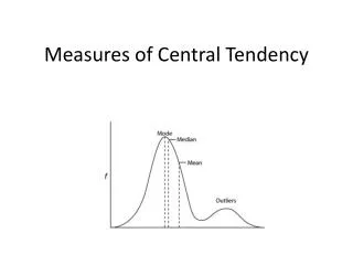
Measures of Central Tendency. Purpose is to describe a distribution’s typical case – do not say “average” case Mode Median Mean (Average). MEASURES OF DISPERSION. Standard deviation Uses every score in the distribution Measures the standard or typical distance from the mean

E N D
Measures of Central Tendency • Purpose is to describe a distribution’s typical case – do not say “average” case • Mode • Median • Mean (Average)
MEASURES OF DISPERSION • Standard deviation • Uses every score in the distribution • Measures the standard or typical distance from the mean • Deviation score = Xi - X • Example: with Mean= 50 and Xi = 53, the deviation score is 53 - 50 = 3
The Problem with Summing Deviations From Mean • 2 parts to a deviation score: the sign and the number • Deviation scores • add up to zero • Because sum of deviations • is always 0, it can’t be • used as a measure of • dispersion X Xi - X 8 +5 1 -2 3 0 0 -3 12 0 Mean = 3
Average Deviation (using absolute value) • Works OK, but… • AD = |Xi – X| N X |Xi – X| 8 5 1 2 3 0 0 3 12 10 AD = 10 / 4 = 2.5 X = 3 Absolute Value to get rid of negative values (otherwise it would add to zero)
Variance & Standard Deviation • Purpose: Both indicate “spread” of scores in a distribution • Calculated using deviation scores • Difference between the mean & each individual score in distribution • To avoid getting a sum of zero, deviation scores are squared before they are added up. • Variance (s2)=sum of squared deviations / N • Standard deviation • Square root of the variance
Terminology • “Sum of Squares” = Sum of Squared Deviations from the Mean = (Xi - X)2 • Variance = sum of squares divided by sample size = (Xi - X)2 = s2 N • Standard Deviation = the square root of the variance = s
Calculating Variance, Then Standard Deviation • Number of credits a sample of 8 students is are taking: • Calculate the mean, variance & standard deviation • Mean = 112/8 = 14 • S2 = 72/8 = 9 • S = 3
Summary Points about the Standard Deviation • Uses all the scores in the distribution • Provides a measure of the typical, or standard, distance from the mean • Increases in value as the distribution becomes more heterogeneous • Useful for making comparisons of variation between distributions • Becomes very important when we discuss the normal curve (Chapter 5, next)
Mean & Standard Deviation Together • Tell us a lot about the typical score & how the scores spread around that score • Useful for comparisons of distributions: • Example: • Class A: mean GPA 2.8, s = 0.3 • Class B: mean GPA 3.3, s = 0.6 • Mean & Standard Deviation Applet
Example Using SPSS Output Statistics Hours watch TV in typical week N Valid 18 Missing 11 Mean 8.2778 Median 5.0000 Mode 5.00 Std. Deviation 7.97648 Variance 63.624 Minimum 1.00 Maximum 28.00 Percentiles 25 3.0000 50 5.0000 75 14.0000 • Hours watching TV for Soc 3155 students: • What is the range & interquartile range? • Is there skew (positive or negative) in this distribution? • What is the most common number of hours reported? • What is the average squared distance that cases deviate from the mean?
THE NORMAL CURVE • Characteristics: • Theoretical distribution of scores • Perfectly symmetrical • Bell-shaped • Unimodal • Continuous • There is a value of Y for every value of X, where X is assumed to be continuous variable • Tails extend infinitely in both directions Y axis x AXIS
THE NORMAL CURVE • Assumption of normality of a given empirical distribution makes it possible to describe this “real-world” distribution based on what we know about the (theoretical) normal curve
THE NORMAL CURVE • .68 of area under the curve (.34 on each side of mean) falls within 1 standard deviation (s) of the mean • In other words, 68% of cases fall within +/- 1 s • 95% of cases fall within 2 s’s • 99% of cases fall within 3 s’s
Areas Under the Normal Curve • Because the normal curve is symmetrical, we know that 50% of its area falls on either side of the mean. • FOR EACH SIDE: • 34.13% of scores in distribution are b/t the mean and 1 s from the mean • 13.59% of scores are between 1 and 2 s’s from the mean • 2.28% of scores are > 2 s’s from the mean
THE NORMAL CURVE • Example: • Male height = normally distributed, mean = 70 inches, s = 4 inches • What is the range of heights that encompasses 99% of the population? • Hint: that’s +/- 3 standard deviations • Answer: 70 +/- (3)(4) = 70 +/- 12 • Range = 58 to 82
THE NORMAL CURVE & Z SCORES • To use the normal curve to answer questions, raw scores of a distribution must be transformed into Z scores • Z scores: Formula: Zi = Xi – X s • A tool to help determine how a given score measures up to the whole distribution RAW SCORES: 66 70 74 Z SCORES: -1 0 1
NORMAL CURVE & Z SCORES • Transforming raw scores to Z scores • a.k.a. “standardizing” • converts all values of variables to a new scale: • mean = 0 • standard deviation = 1 • Converting raw scores to Z scores makes it easy to compare 2+ variables • Z scores also allow us to find areas under the theoretical normal curve
Xi = 120; X = 100; s=10 Z= 120 – 100 = +2.00 10 Xi = 80, S = 10 Xi = 112, S = 10 Xi = 95; X = 86; s=7 Z= 80 – 100 = -2.00 10 Z = 112 – 100 = 1.20 10 Z= 95 – 86 = 1.29 7 Z SCORE FORMULA Z = Xi – X S
USING Z SCORES FOR COMPARISONS • Example 1: • An outdoor magazine does an analysis that assigns separate scores for states’ “quality of hunting” (MN = 81) & “quality of fishing” (MN =74). Based on the following information, which score is higher relative to other states? • Formula: Zi = Xi – X s • Quality of hunting for all states: X = 69, s = 8 • Quality of fishing for all states: X = 65, s = 5 • Z Score for “hunting”: 81 – 69 = 1.5 8 • Z Score for “fishing”: 73 – 65 = 1.6 5 • CONCLUSION: Relative to other states, Minnesota’s “fishing” score was higher than its “hunting” score.
USING Z SCORES FOR COMPARISONS • Example 2: • You score 80 on a Sociology exam & 68 on a Philosophy exam. On which test did you do better relative to other students in each class? Formula: Zi = Xi – X s • Sociology: X = 83, s = 10 • Philosophy: X = 62, s = 6 • Z Score for Sociology: 80 – 83 = - 0.3 10 • Z Score for Philosophy: 68 – 62 = 1 6 • CONCLUSION: Relative to others in your classes, you did better on the philosophy test
Normal curve table • For any standardized normal distribution, Appendix A (p. 453-456) of Healey provides precise info on: • the area between the mean and the Z score (column b) • the area beyond Z (column c) • Table reports absolute values of Z scores • Can be used to find: • The total area above or below a Z score • The total area between 2 Z scores
THE NORMAL DISTRIBUTION • Area above or below a Z score • If we know how many S.D.s away from the mean a score is, assuming a normal distribution, we know what % of scores falls above or below that score • This info can be used to calculate percentiles
AREA BELOW Z • EXAMPLE 1: You get a 58 on a Sociology test. You learn that the mean score was 50 and the S.D. was 10. • What % of scores was below yours? Zi = Xi – X = 58 – 50 = 0.8 s 10
AREA BELOW Z • What % of scores was below yours? Zi = Xi – X = 58 – 50 = 0.8 s 10 • Appendix A, Column B -- .2881 (28.81%) of area of normal curve falls between mean and a Z score of 0.8 • Because your score (58) > the mean (50), remember to add .50 (50%) to the above value • .50 (area below mean) + .2881 (area b/t mean & Z score) = .7881 (78.81% of scores were below yours) • YOUR SCORE WAS IN THE 79TH PERCENTILE FIND THIS AREA FROM COLUMN B
AREA BELOW Z • Example 2: • Your friend gets a 44 (mean = 50 & s=10) on the same test • What % of scores was below his? Zi = Xi – X = 44 – 50 = - 0.6 s 10
AREA BELOW Z • What % of scores was below his? Z= Xi – X = 44 – 50= -0.6 s 10 • Appendix A, Column C -- .2743 (27.43%) of area of normal curve is under a Z score of -0.6 • .2743 (area beyond [below] his Z score) 27.43% of scores were below his • YOUR FRIEND’S SCORE WAS IN THE 27TH PERCENTILE FIND THIS AREA FROM COLUMN C
Z SCORES: “ABOVE” EXAMPLE • Sometimes, lower is better… • Example: If you shot a 68 in golf (mean=73.5, s = 4), how many scores are above yours? 68 – 73.5 = - 1.37 4 • Appendix A, Column B -- .4147 (41.47%) of area of normal curve falls between mean and a Z score of 1.37 • Because your score (68) < the mean (73.5), remember to add .50 (50%) to the above value • .50 (area above mean) + .4147 (area b/t mean & Z score) = .9147 (91.47% of scores were above yours) 68 73.5 FIND THIS AREA FROM COLUMN B
Area between 2 Z Scores • What percentage of people have I.Q. scores between Stan’s score of 110 and Shelly’s score of 125? (mean = 100, s = 15) • CALCULATE Z SCORES
AREA BETWEEN 2 Z SCORES • What percentage of people have I.Q. scores between Stan’s score of 110 and Shelly’s score of 125? (mean = 100, s = 15) • CALCULATE Z SCORES: • Stan’s z = .67 • Shelly’s z = 1.67 • Proportion between mean (0) & .67 = .2486 = 24.86% • Proportion between mean & 1.67 = .4525 = 45.25% • Proportion of scores between 110 and 125 is equal to: • 45.25% – 24.86% = 20.39% 0 .67 1.67
AREA BETWEEN 2 Z SCORES • EXAMPLE 2: • If the mean prison admission rate for U.S. counties was 385 per 100k, with a standard deviation of 151 (approx. normal distribution) • Given this information, what percentage of counties fall between counties A (220 per 100k) & B (450 per 100k)? • Answers: • A: 220-385 = -165 = -1.09 151 151 B: 450-385 = 65 = 0.43 151 151 County A: Z of -1.09 = .3621 = 36.21% County B: Z of 0.43 = .1664 = 16.64% Answer: 36.21 + 16.64 = 52.85%
4 More Sample Problems • For a sample of 150 U.S. cities, the mean poverty rate (per 100) is 12.5 with a standard deviation of 4.0. The distribution is approximately normal. • Based on the above information: • What percent of cities had a poverty rate of more than 8.5 per 100? • What percent of cities had a rate between 13.0 and 16.5? • What percent of cities had a rate between 10.5 and 14.3? • What percent of cities had a rate between 8.5 and 10.5?