Download
1 / 25
250 likes | 443 Views
A Conjugate Gradient-based BPTT-like Optimal Control Algorithm. Josip Kasać*, Joško Deur*, Branko Novaković*, Ilya Kolmanovsky** * University of Zagreb, Faculty of Mech. Eng. & Naval Arch., Zagreb, Croatia (e-mail: josip.kasac@fsb.hr, josko.deur@fsb.hr, branko.novakovic@fsb.hr).

E N D
A Conjugate Gradient-based BPTT-like Optimal Control Algorithm Josip Kasać*, Joško Deur*, Branko Novaković*, Ilya Kolmanovsky** *University of Zagreb, Faculty of Mech. Eng. & Naval Arch., Zagreb, Croatia(e-mail: josip.kasac@fsb.hr, josko.deur@fsb.hr, branko.novakovic@fsb.hr). ** Ford Research Laboratory, Dearborn, MI 48121-2053 USA (e-mail: ikolmano@ford.com).
Introduction • In this paper a gradient-based algorithm for optimal control of nonlinear multivariable systems with control and state vectors constraints is proposed • The algorithm has a backward-in-time recurrent structure similar to the backpropagation-through-time (BPTT) algorithm • Original algorithm (Euler method and standard gradient algorithm) is extended with: • implementation of higher-order Adams methods • implementation of conjugate gradient methods • Vehicle dynamics control example–double lane change maneuver executed by using control actions of active rear steering and active rear differential actuators.
Continuous-time optimal control problem formulation • Find the control vectoru(t) Rm that minimizes the cost function • subject to the nonlinear MIMO dynamics process equations • with initial and final conditions of the state vector • subject to control & state vector inequality and equality constraints
Extending the cost function with constraints-related terms • Reduced optimal control problem - find u(t) that minimizes: • subject to the process equations (only): • where penalty terms are introduced:
Transformation to terminal optimal control problem • In order to simplify application of higher-order numerical integration methods, an additional state variable is introduced: • The final continuous-time optimization problem - find the control vector u(t) that minimizes the terminal condition: • subject to the process equations: • where:
Multistep Adams methods 1st order Adamsmethod(Euler method): 2nd order Adamsmethod: 3rd order Adamsmethod: k-th order Adamsmethod:
State-space representation ofthe Adams methods 3rd order Adamsmethod: The fourth-order Runge-Kutta method is used (only) for calculation of the first k initial conditions for the k-th order Adams method: Initial conditions: • The Adams method of k-th order requires only one computations of the function f(i) in a sampling time ti • The Runge-Kutta method of k-th order requires thek computations of the functionf(i) in a sampling time ti
State-space representation of theAdams methods k-th order Adamsmethod: Initial conditions: • The k-th order Adams discretization of continuous process equations: • where: • Adams method provide same state-space formulation of the optimal control problem as Euler method: • Runge-Kutta method leads to:
Discrete–time optimization problem • Thefinal discrete-time optimization problem - find the control sequence u(0), u(1), u(2),…, u(N-1) that minimizes the terminal cost function: • subject to the discrete-time process equations (k-th order Adams method): • Gradient algorithm: • The cost function J depends explicitly only on the state vector at the terminal time x(N) • implicit dependence on u(0), u(1), u(2),…, u(N-1) follows from the discrete-time state equations
Exact gradient calculation • Implicit but exact calculation of cost function gradient The partial derivatives canbe calculated backward in time • for i=N-1: • for i=N-2: • chain rule for ordered derivatives →back-propagation-through-time (BPTT)algorithm
The final algorithm for gradient calculation • Initialization (i=N-1): • Backward-in-time iterations (i=N-2, N-3, ..., 1, 0): • where and are Jacobians with elements: • and where:
Conjugate gradient methods • d(k) – search direction vector • g(k)– gradient • Standard gradient algorithm: βk=0 and ηk = const. • Gradient algorithm with momentum:βk=const. • Standard method for computing ηk is line search algorithm which requires one-dimensional minimization of the cost function. • Computationally expensive method - require many evaluations of the cost function during one iteration of the gradient algorithm.
Learning rate adaptation • Learning rate adaptation (a modified version of SuperSAB algorithm): • Fletcher-Reeves: • Polak-Ribiere: • Hestenes-Stiefel: • Dai-Yuan:
Active Front d x Steering f D = t T 0 f y t T 2 1 f T D Central T i b c Power Differential Plant U V l CoG State r Active Rear Variables Steering T d r r c Rear D T Differential r x y 3 4 z t / 2 t / 2 Vehicle dynamics control
1. State-Space Subsystem • 1.1 Longitudinal, lateral, and yaw DOF Fxi,Fyi,- longitudinal and lateral forces M- vehicle mass, Izz- vehicle moment of inertia, b - distance from the front axle to the CoG, c - distance from the rear axle to the CoG, t - track U, V - longitudinal and lateral velocity, r - yaw rate, X,Y - vehicle position in the inertial system ψ - yaw angle
1.2 The wheel rotational dynamics j- rotational speed of the i-th wheel, Fxti - longitudinal force of the i-th tire, Ti - torque at the i-th wheel, Iwi- wheel moment of inertia, R - effective tire radius. • 1.3 Delayed total lateral force (needed to calculate the lateraltire load shift): • 1.4 The actuator dynamics: - rear wheel steering angle, - rear differential torque shift, - actuator time constants.
2. Longitudinal and Lateral Slip Subsystem 3. TireLoad Subsystem l - wheelbase hg - CoG height 4. Tire Subsystem μ- tire friction coefficient B, C,D - tire model parameters 5. Rear Active Differential Subsystem ΔTr - differential torque shift control variable, Ti - input torque (driveline torque) and Tb - braking torque
GCC optimization problem formulation • Nonlinear vehicle dynamics description: • Control variables (to be optimized): r(ARS) and Tr(TVD/ALSD) • Other inputs (driver’s inputs): f • State variables: U, V, r, i(i = 1,...,4), , X, Y • Cost functions definitions: Reference trajectory • Path following(in external coordinates): • Control effort penalty: • Different constraints implemented: • control variable limit: • vehicle side slip angle limit: • boundary condition on Y and dY / dt:
Simulation results – double line change maneuver • Front wheel steering optimization results for asphalt road ( = 1) using Euler and 2nd order Adams methods:
Simulation results – double line change maneuver • Optimization results for ARS+TVD control and = 0.6 usingEuler and 2nd order Adams methods :
Comparison of gradient methods • Convergence properties for the double-line change example (M=400):
Comparison of gradient methods • Comparison of standard gradient algorithm (M=4000) with CG algorithms (M=400): • for a similar level of accuracy theconjugate gradients methods are about10 times faster then the standard gradient algorithm
Comparison of gradient methods • The number of iterations and computational time for the similar level of accuracy: • for a similar level of accuracy theconjugate gradientsmethods Dai-Yuan andHestenes-Stiefel are about 23 times faster then the standard gradient algorithm
Sensitivity of the CG algorithm • CG algorithm contains four free parameters:η0,d¯, d+,βmax • For the parameters, d¯, d+,βmax, tuning region is known in advance • Initial learning rateη0 is dependent on specific optimization problem • CG method are less sensitive to the choice of η0 then the standard gradient algorithm
Conclusions • A back-propagation-through-time (BPTT) exact gradient method for optimal control has been applied for control variable optimization in Global Chassis Control (GCC) systems. • The BPTT optimization approach is proven to be numerically robust, precise, and computationally efficient • Recent model extensions: • model extension with roll, pitch, and heave dynamics(full 10-DOF model) • use of more accurate tire model(full Magic formula tire model) • introduction of a driver model for closed-loop maneuvers • The future work will be directed towards: • combined control/parameter optimization • feedback systems optimization • differential game controller