Download
1 / 41
420 likes | 1.09k Views
Polygon Triangulation Guarding an Art Gallery Introduction Works of famous painters are not only popular among art lovers, but also among criminals. They are very valuable, easy to transport, and apparently not so difficult to sell.

E N D
Polygon Triangulation Guarding an Art Gallery
Introduction • Works of famous painters are not only popular among art lovers, but also among criminals. They are very valuable, easy to transport, and apparently not so difficult to sell. • Art galleries therefore have to guard their collections carefully. • During the day the attendants can keep a look-out, but at night this has to be done by video cameras. • The images from the cameras are sent to TV screens in the office of the night watch. Because it is easier to keep an eye on few TV screens rather than on many, the number of cameras should be as small as possible. • An additional advantage of a small number of cameras is that the cost of the security system will be lower. • On the other hand we cannot have too few cameras, because every part of the gallery must be visible to at least one of them. So we should place the cameras at strategic positions, such that each of them guards a large part of the gallery.
Defining the art gallery problem more precisely • A gallery is, of course a 3-dimensional space, but a floor plan gives us enough information to place the cameras. • Therefore we model a gallery as a polygonal region in the plane. • We further restrict ourselves to regions that are SIMPLE POLYGONS, that is, regions enclosed by a single closed polygonal chain that does not intersect itself. Thus we do not allow regions with holes. • A camera position in the gallery corresponds to a point in the polygon. A camera sees those points in the polygon to which it can be connected with an open segment that lies in the interior of the polygon.
How many cameras do we need to guard a simple polygon • This clearly depends on the polygon at hand: the more complex the polygon, the more cameras are required. • We shall therefore express the bound on the number of cameras needed in terms of n, the number of vertices of the polygon. • But even when two polygons have the same number of vertices, one can be easier to guard than the other. A convex polygon (in fact a star-shaped polygon), for example can always be guarded with one camera. • To be on the safe side we shall look at the worst-case scenario, that is, we shall give a bound that is good for any simple polygon with n vertices. • It would be nice if we could find the minimum number of cameras for the specific polygon we are given, not just a worst-case bound. Unfortunately the problem of finding the minimum number of cameras for a given polygon is NP-hard.
Decomposing a simple polygon • Let P be a simple polygon with n vertices. • Because P may be a complicated shape, it seems difficult to say anything about the number of cameras we need to guard P. • Hence, we first decompose P into pieces that are easy to guard, namely triangles. • We do this by drawing DIAGONALS between pairs of vertices. • A diagonal is an open line segment that connects two vertices of P and lies in the interior of P. • A decomposition of a polygon into triangles by a maximal set of non-intersecting triangles is called a TRIANGULATION.
Triangulations • Triangulations are usually not unique. • We can guard P by placing a camera in every triangle of a triangulation T(P) of P. • But does a triangulation always exist? • And how many triangles can there be in a triangulation? • THEOREM: Every simple polygon admits a triangulation, and any triangulation of a simple polygon with n vertices consists of exactly n-2 triangles.
Proof of the Theorem • We prove this theorem by induction on n. When n=3 the polygon itself is a triangle and the theorem is trivially true. Let n>3, and assume that the theorem is true for all m<n. • Let P be a polygon with n vertices. We first prove the existence of a diagonal in P. Let v be the leftmost vertex of P. Let u and w be its neighbors. If the open segment uw lies in the interior of P we have found a diagonal. • Otherwise there are one or more vertices inside the triangle defined by u,v and w, or on the diagonal uw. Of those vertices let v’ be the one farthest from uw. The segment connecting v’ to v cannot intersect an edge of P. hence vv’ is a diagonal. • Any diagonal cuts P into two simple subpolygons, and both of them can be triangulated by the induction assumption.
Reducing the number of cameras • Last Theorem implies that any simple polygon with n vertices can be guarded with n-2 cameras. • But placing a camera inside every triangle seems overkill. A camera placed on a diagonal, for example, will guard two triangles, so by placing the cameras on well-chosen diagonals we might be able to reduce the number of cameras to roughly n/2. • Placing cameras at vertices seems even better, because a vertex can be incident to many triangles, and a camera at that vertex guards all of them.
3-coloring of a triangulated polygon • Let T(P) be a triangulation of P. Select a subset of the vertices of P, such that any triangle in T(P) has at least one selected vertex, and place the cameras at the selected vertices. • To find such a subset we assign each vertex of P a color: red, green, or blue. The coloring will be such that any two vertices connected by an edge or a diagonal have different colors. This is called a 3-COLORING OF A TRIANGULATED POLYGON. • In such 3-colorings, every triangle has a red, a green, and a blue vertex. Hence if we place cameras at all green vertices, say, we have guarded the whole polygon. • By choosing the smallest color class to place the cameras, we can guard P using at mostn/3 cameras.
Does a 3-coloring always exist? • The answer is yes. To see this, we look at what is called the DUAL GRAPH of T(P). • This graph G(T(P)) has a node for every triangle in T(P). We denote the triangle corresponding to a node v by t(v). There is an arc between two nodes v and w if t(v) and t(w) share a diagonal. • The arcs in G(T(P)) correspond to diagonals in T(P). Because any diagonal cuts P into two, the removal of an edge from G(T(P)) splits the graph into two. Hence G(T(P)) is a tree. • This means that we can find a 3-coloring using a simple graph traversal.
Finding a 3-coloring using a simple graph traversal • We start from any node. This node corresponds to a triangle and we color the three vertices of this triangle with colors red, green and blue. • Now we follow one edge of the grapf till we reach another node; the two triangles correspondinf to the wo nodes share a diagonal, so two of the vertices of the second triangle have already been colored, and there is only one color left for the third vertex of the second triangle. • As G(T(P)) is a tree, each node is visited only one time.
Can we improve n/3 ? • We conclude that a triangulated simple polygon can always be 3-colored. • As a result, any simple polygon can be guarded with n/3 cameras. But perhaps we can do even better. After all, a camera placed at a vertex may guard more than just the incident triangles. • Unfortunately, for any n there are simple polygons that require n/3 cameras. An example is a comb-shaped polygon with a long horizontal base edge and n/3 prongs made of two edges each. The prongs are connected by horizontal edges. The construction can be made such that there is no position in the polygon from which a camera can look into two prongs of the comb simultaneously. • So we cannot hope for a strategy that always produces less than n/3 cameras. In other words, the 3-coloring approach is optimal in the worst case.
Art Gallery Theorem • So we just proved the Art Gallery Theorem, a classical result from combinatorial geometry. • THEOREM: For a simple polygon with n vertices, n/3 cameras are ocasionally necessary and always sufficient to have every point in the polygon visible from at least one of the cameras.
What about an algorithm? • Now we know that n/3 cameras are always suficient. But we don’t have an efficient algorithm to compute the camera positions yet. • What we need is a fast algorithm for triangulating a simple polygon. The algorithm should deliver a suitable representation of the triangulation –a doubly-connected edge list, for instance- so that we can step in constant time from a triangle to its neighbors. • Given such a representation, we can compute a set of at most n/3 camera positions in linear time with the method described above: use depth first search on the dual graph to compute a 3-coloring and take the smallest color class to place the cameras. • In the coming sections we describe how to compute a triangulation in O(n logn) time. Anticipating this, we already state the final result about guarding a polygon:THEOREM: Let P be a simple polygon with n vertices. A set of n/3 camera positions in P such that any point inside P is visible from at least one of the cameras can be computed in O(n logn) time.
A First Approach to the Algorithm • Let P be a simple polygon with n vertices. We saw that a triangulation of P always exist. The proof of this fact is constructive and leads to a recursive triangulation algorithm: find the diagonal and triangulate the two resulting subpolygons recursively. • To find the diagonal we take the leftmost vertex v of P and try to connect its two neighbors u and w; if this fails we connect v to the vertex farthest from uv inside the triangle defined by u,v, and w. • This way it takes linear time to find a diagonal. This diagonal may split P into a triangle and a polygon with n-1 vertices. As a consequence, the triangulation algorithm will take quadratic time in the worst case (n+(n-1)+ … + 3=(n+3)(n-2)/2). • Can we do better? For some classes of polygons we surely can. Convex polygons, for instance, are easy: pick one vertex of the polygon and draw diagonals from this vertex to all other vertices except its neighbors. This takes only linear time. So a possible approach to triangulate a non-convex polygon would be to first decompose P into convex pieces, and then triangulate the pieces. Unfortunately, it is as difficult to partition a polygon into convex pieces as it is to triangulate it. • Therefore we shall decompose P into so-called MONOTONE pieces, which turns out to be a lot easier.
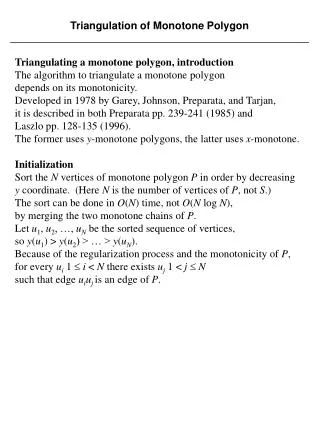
Monotone Polygons • A simple polygon is called MONOTONE with respect to a line l if for any line l’ perpendicular to l the intersection of the polygon with l’ is connected. • A polygon that is monotone with respect to the y-axis is called y-monotone. • The following property is characteristic for y-monotone polygons: if we walk from a topmost to a bottommost vertex along the left (or the right) boundary chain, then we always move downwards or horizontally, never upwards.
Strategy • Our strategy to triangulate the polygon P is to first partition P into y-monotone pieces, and then triangulate the pieces. • We can partition a polygon into monotone pieces as follows: Imagine walking from the topmost vertex of P to the bottom vertex on the left or right boundary chain. A vertex where the direction in which we walk switches from downward to upward or from upward to downward is called a TURN VERTEX. To partition P into y-monotone pieces we should get rid of these TURN VERTICES. This can be done by adding diagonals. If at a turn vertex v both incident edges go down and the interior of the polygon locally lies above v, then we must choose a diagonal that goes up from v. The diagonal splits the polygon into two. The vertex v will appear in both pieces. Moreover, in both pieces v has an edge going down (namely an original edge of P) and an edge going up (the diagonal). Hence, v cannot be a turn vertex anymore in either of them. If both incident edges of a turn vertex go up and the interior locally lies below it, we have to choose a diagonal that goes down.
Analysing turn vertices • If we want to define the different types of turn vertices carefully, we should pay special attention to vertices with equal y-coordinate. • We do this by defining the notions of “below” and “above” as follows: • A point p is below another point q if py<qy or py=qy and px>qx, and p is above q if py>q y or py=qy and px<qx. • We distinguish five types of vertices in P. Four of these types are TURN vertices: START vertices, SPLIT vertices, END vertices and MERGE vertices. They are defined as follows: A vertex v is a START VERTEX if its two neighbors lie below it an the interior angle at v is less than ; if the interior angle is greater than then v is a SPLIT VERTEX. (If both neighbors lie below v , then the interior angle cannot be exactly .) A vertex is an END VERTEX if its two neighbors lie above it and the interior angle at v is less than ; if the interior angle is greater than then v is a MERGE VERTEX. The vertices that are not turn vertices are REGULAR VERTICES. Thus a regular vertex has one of its neighbors above it, and the other neighbor below it. • These names have been chosen because the algorithm will use a downward plane sweep, maintaining the intersection of the sweep line with the polygon. When the sweepline reaches a split vertex, a component of the intersection splits, when it reaches a merge vertex, two components merge, and so on.
Different types of vertices v3 start vertex v5 e3 e5 e4 end vertex v6 v4 e2 e6 regular vertex v7 v9 e7 split vertex v2 e8 v1 v8 e1 merge vertex e9 v14 e15 e14 v10 e13 v15 e10 e12 e11 v12 v13 v11
Split and merge vertices • The split and merge vertices are sources of local non-monotonicity. The following, stronger statement is even true: • LEMMA: A polygon is Y-monotone if it has no split vertices or merge vertices.
Spilt vertex Suppose that the swap line reachs a spilt vertex vi. Let ej be the edge immediately to the left of vi on the sweep line, and let ek be the edge immediately to the right of vi on the sweep line. Then we can always connect vi to the lowest vertex in between ej and ek, and above vi. helper(ej) ej ek vi l ei-1 ei
Merge vertex Suppose that the swap line reachs a merge vertex vi. Let ej and ek be the edges immediately to the left and to the left of vi on the sweep line. Observe that vi becomes the new helper of ej when we reach it. We would like to connect vi to the highest vertex below the sweep line in between ej and ek. ej ek vi vm
Getting rid of split and merge vertices. • The above lemma implies that a polygon P has been partitioned into y-monotone pieces once we get rid of its split and merge vertices. • We do this by adding a diagonal going upward from each split vertex and a diagonal going downward from each merge vertex. These diagonals should not intersect each other. Once we have done this, P has been partitioned into y-monotone pieces. • Let vi be a split vertex and let ej be the edge immediately to the left of vi on the sweep line. The helper of vi is the lowest vertex above the sweep line such that the horizontal segment connecting the vertex to the segment ej lies inside P.
ALGORITHM: MakeMonotone(P) • INPUT: A simple polygon P stored in a doubly-connected edge list D. • OUTPUT: A partitioning of P into monotone subpolygons, stored in D. • Construct a priority queue Q on the vertices of P, using their y-coordinates as priority. If two points have the same y-coordinate, the one with smaller x-coordinate has higher priority. • Initialize an empty binary search tree T. • WHILE Q is not empty • DO Remove the vertex vi with the highest priority from Q • Call the appropriate procedure to handle the vertex, depending on its type.
HandleStartVertex(vi) • Insert ei in T and set helper(ei) to vi.
HandleEndVertex(vi) • IF helper(ei-1) is a merge vertex • THEN Insert the diagonal connecting vi to helper(ei-1) in D. • Delete ei-1 from T.
HandleSplitVertex(vi) • Search in T to find the edge ej directly left of vi. • Insert the diagonal connecting vi to helper(ej) in D. • Helper(ej) vi • Insert ei in T and set helper(ei) to vi.
HandleMergeVertex(vi) 1. IF helper(ej-1) is a merge vertex 2. THEN Insert the diagonal connecting vi to helper(ej-1) in D. 3. Delete ej-1 from T. 4. Search in T to find the edge ej directly left of vi. 5. IF helper(ej) is a merge vertex 6. THEN Insert the diagonal connecting vi to helper(ej) in D. 7. helper(ej) vi.
HandleRegularVertex(vi) • IF the interior of P lies to the right of vi • THEN IF helper(ei-1) is a merge vertex • THEN Insert the diagonal connecting vi to helper(ei-1) in D. • Delete ei-1 from T. • Insert ei in T and set helper(ei) to vi. • ELSE Search in T to find the edge ej directly left of vi. • IF helper(ej) is a merge vertex • THEN Insert the diagonal connecting vi to helper(ej) in D. • helper(ej) vi.
Triangulating a Monotone Polygon. • To partition a simple polygon into y-monotone pieces take O(n logn) time. • In itself is not very interesting, but we are going to show that monotone polygons can be triangulated in linear time. • Together these results imply that any simple polygon can be triangulated in O(n logn) time, a nice improvement over the quadratic time algorithm that we sketched at the beginning.
ALGORITHM: TriangulateMonotonePolygon(P) • INPUT: A strictly y-monotone polygon P Initializestored in a doubly-connected edge list D. • OUTPUT: A triangulation of P stored in the doubly-connected edge list D. • Merge the vertices on the left chain and the vertices on the right chain of P into one sequence, sorted on decreasing y-coordinate. If two vertices have the same y-coordinate, then the leftmost one comes first. Let u1, u2, … , un denote the sorted sequence. • Initialize an empty stack S, and push u1 and u2 onto it. • FOR j3 to n-1 DO IF uj and the vertex on top of S are on different chains • THEN Pop all vertices from S. • Insert into D a diagonal from uj to each popped vertex, except the last one. • Push uj-1 and uj onto S. • ELSE Pop one vertex from S. • Pop the other vertices from S as long as the diagonals from uj to them are inside P. Insert these diagonals into D. Push the last vertex that has been popped back onto S. Push uj onto S. • Add diagonals from u to all stack vertices except the first and the last one.
a S[a] b S[b,a] S[a] S[b,a] S[c,b,a] c d S[b,a] S[c,b,a] S[d,c,b,a] e S[] S[e,b]
a S[a] S[b,a] b c S[a] S[b,a] S[c,b,a] d S[b,a] S[c,b,a] S[d,c,b,a] e S[c,b,a] S[d,c,b,a] S[e,d,c,b,a] f S[] S[f,e]
v3 start vertex v5 e3 e5 e4 end vertex v6 v4 e2 e6 regular vertex v7 v9 e7 split vertex v2 e8 v1 v8 e1 merge vertex e9 v14 e15 e14 v10 e13 v15 e10 e12 e11 v12 v13 v11
m v