Download
1 / 59
610 likes | 838 Views
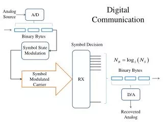
Lecture 6 Digital Communication. Dr. Rashid Saleem. Sampling Theorem. Where f s ≥ 2f m and t 0 = 2 p / f s Therefore . and. By comparing these two equations, if t = -n/ f s.

E N D
Lecture 6Digital Communication Dr. Rashid Saleem
Sampling Theorem Where fs≥ 2fm and t0 = 2p/fs Therefore and By comparing these two equations, if t = -n/fs This says that we can obtain each Cn from the sample value of m(t) at time t = - n/fs. Once Cn is known, we can obtain Mp(f), and once Mp(f) is known, we can obtain m(t).
Signal Reconstruction The process of reconstructing an analogue signal m(t) from its samples is known as interpolation. Mn(f) be the Fourier transform of the nth sample m( n/fs). If t << 1/ fs , m(t) can be assumed to be constant over the sampling time, the analogue signal can be recovered by using a low-pass filter with a cutoff frequency of fs /2 (≥ fm). Assume that the ideal low-pass filter has the transfer function H(f) = Ke-j2pftd , where K is a constant and td is a time delay. Without loosing the generality, the filter gain can be K = 1 and the filter delay td = 0.
Signal Reconstruction Let gn(t) be the filter output response to the nth input sample m( n/fs). The Fourier transform of g n (t) is Gn(f) = H(f)Mn(f) = Mn(f) and This yields values of g(t) between samples as a weighted sum of all sample values. g(t) is not only defined at the sampling instants, but it is proportional to m(t) at all instants of time.
8 Analog PAM 6 4 2 0 -2 -4 -6 -0.5 0 0.5 1 1.5 2 2.5 3 3.5 4 time Sample & HoldPulse Amplitude Modulation
Pulse Amplitude Modulation The sampling theorem is very important because it allows us to replace an analogue signal by a discrete sample and reconstruct the analogue signal from its sample values. It opens doors to many new techniques of communicating analogue signal by samples. A system transmitting sample values of the analogue signal is called a pulse amplitude modulation (PAM) system
Time Division Multiplexing (TDM) • To allows signals from many users to be transmitted simultaneously over a single communication channel. • We see from the sampling process that, with t << Ts, there is a time gap between two consecutive samples in a single-user PAM system. • Suppose that we have several different signals of the same or different bandwidth. If we sample the signals in a sequential manner, we can put the samples in the time gaps. • All these signal samples can now be transmitted along a single communication channel. • At the receiving end, the signals can be separated and recovered. We now have a time-multiplexed system. • Such a multiplexing technique is called time division multiplexing (TDM).
Aliasing • If fs < 2B, the waveform is “undersampled” • “aliasing” or “spectral folding” • How can we avoid aliasing? • Increase fs • “Pre-filter” the signal so that it is bandlimited to 2B < fs
Quantization Mapping • Quantization • Dequantization Continuous values Binary codes Binary codes Continuous values
Quantization • Sampling results in a series of pulses of varying amplitude values ranging between two limits: a min and a max. • The amplitude values are infinite between the two limits. • We need to map the infinite amplitude values onto a finite set of known values. • This is achieved by dividing the distance between min and max into Lzones, each of height = (max - min)/L
QuantizationLevels • The midpoint of each zone is assigned a value from 0 to L-1 (resulting in L values) • Each sample falling in a zone is then approximated to the value of the midpoint.
Quantization Zones • Assume we have a voltage signal with amplitudes Vmin=-20V and Vmax=+20V. • We want to use L=8 quantization levels. • Zone width = (20 - -20)/8 = 5 • The 8 zones are: -20 to -15, -15 to -10, -10 to -5, -5 to 0, 0 to +5, +5 to +10, +10 to +15, +15 to +20 • The midpoints are: -17.5, -12.5, -7.5, -2.5, 2.5, 7.5, 12.5, 17.5
Assigning Codes to Zones • Each zone is then assigned a binary code. • The number of bits required to encode the zones, or the number of bits per sample as it is commonly referred to, is obtained as follows: nb = log2L = log28 = log223 = 3 log22= 3x1 = 3 • Given our example, nb = 3 • The 8 zone (or level) codes are therefore: 000, 001, 010, 011, 100, 101, 110, and 111 • Assigning codes to zones: • 000 will refer to zone -20 to -15 • 001 to zone -15 to -10, etc. etc.
Quantization Error • When a signal is quantized, we introduce an error - the coded signal is an approximation of the actual amplitude value. • The difference between actual and coded value (midpoint) is referred to as the quantization error. • The more zones, the smaller which results in smaller errors. • BUT, the more zones the more bits required to encode the samples -> higher bit rate
Quantization Error and SNQR • Signals with lower amplitude values will suffer more from quantization error as the error range: /2, is fixed for all signal levels. • Non linear quantization is used to alleviate this problem. Goal is to keep SNQR fixed for all sample values. • Two approaches: • The quantization levels follow a logarithmic curve. Smaller ’s at lower amplitudes and larger’s at higher amplitudes.
Bit rate and bandwidth requirements of PCM • Companding: The sample values are compressed at the sender into logarithmic zones, and then expanded at the receiver. The zones are fixed in height. • The bit rate of a PCM signal can be calculated from the number of bits per sample x the sampling rate Bit rate = nb x fs • The bandwidth required to transmit this signal depends on the type of line encoding used. • A digitized signal will always need more bandwidth than the original analog signal. • Price we pay for robustness and other features of digital transmission.
Digitization of Audio Samples Quantization • Audio signals are continuous in time and amplitude • Audio signal must be digitized in both time and amplitude to be represented in binary form. • Discrete in time by sampling – Nyquist • Discrete in amplitude by quantization • Once samples have been captured, they must be made discrete in amplitude. A to D Converter (Amplitude Quantizer) Zero Order Hold (Time Quantizer) Digital Bitstream output Analog Signal Input Step 2: Quantization Step 1: Sampling The two step digitization process
Quantization • An analogue signal can be converted into a digital signal by the use of sampling and quantization. • Quantization is the process in which the sampled values of an analogue signal are converted into discrete levels. • The quality of reconstructing the analogue waveform from a set of samples depends on fineness of the quantization process. • The difference between the quantized level and the original analogue signal sample results in quantized noise. • The mean square quantized noise relates to the performance in terms of signal-to-quantized-noise and is dependent on statistical character of the input signal.
Quantization • Quantization • Converts actual sample values (usually voltage measurements) into an integer approximation • Process of rounding off a continuous value so that it can be represented by a fixed number of binary digits • Tradeoff between number of bits required and error • Human perception limitations affect allowable error • Specific application affects allowable error • Two approaches to quantization • Rounding the sample to the closest integer. • (e.g. round 3.14 to 3) • Create a Quantizer table that generates a staircase pattern of values based on a step size.
Quantization • Consider an audio signal with a voltage range between -10 and +10 • Assume the audio waveform has already been time sampled, as shown • How can the amplitude also be converted into discrete values?
For this example, let’s choose to represent each sample by 4 bits • There are an infinite number of voltages between -10 and 10. • We will have to assign a range of voltages to each 4-bit codeword. • There will be 16 levels. • How large will each step be?
Quantization • Input to the quantizer is continuous and have infinite amplitude range. • Output of the quantizer is discrete and finite range of amplitudes. • There are two types of quantizations: Uniform and non uniform.
QuantizationProcess • A continuous signal, such as voice, has a continuous range of amplitudes and therefore its samples have a continuous amplitude range. In other words, within the finite amplitude range of the signal, we find an infinite number of amplitude levels. • It is not necessary in fact to transmit the exact amplitudes of the samples. • Any human sense (the ear or the eye), as ultimate receiver, can detect only finite intensity differences. This means that the original continuous signal may be approximated by a signal constructed of discrete amplitudes selected on a minimum error basis from an available set.
QuantizationProcess • The existence of a finite number of discrete amplitude levels with sufficiently close spacing, we may make the approximated signal practically indistinguishable from the original continuous signal. • Amplitude quantization is defined as the process of transforming the sample amplitude m(nTs) of a baseband message signal m(t) at time t=nTs into a discrete amplitude v(nTs) taken from a finite set of possible levels. • We assume that the quantization process is memoryless and instantaneous, which means that the transformation at time t=nTs is not affected by earlier or later samples of the message signal. • This simple form of scalar quantization, though not optimum, is commonly used in practice.
QuantizationProcess • When dealing with a memoryless quantizer, we may simplify the notation by dropping the time index. • We may thus use the symbol m in place of m(nTs), as indicated in the block diagram of a quantizer shown as under: • Then, as shown under, the signal amplitude m is specified by the index k if it lies inside the partition cell Where L is the total number of amplitude levels used in the quantizer.
QuantizationProcess • The discrete amplitudes mk, k = 1, 2, …, L, at the quantizer input are called decision levels or decision thresholds. • At the quantizer output, the indexk is transformed into an amplitude vk that represents all amplitudes of the cell Ik; the discrete amplitudes vk, k=1,2,3,……,L, are called representation levels or reconstruction levels, and the spacing between two adjacent representation levels is called a quantum or step size. • Thus, the quantizer output v equals vkif the input signal sample m belongs to the interval Ik. • The mapping v=g(m) is the quantizer characteristic, which is a staircase function by definition.
Quantizing • Let Message signal be m(t) having amplitude in the range (-mp to mp) i.e peak to peak voltage is 2mpwith L quantized levels. is the signal reconstructed from quantized samples. • The distortion q (t) in the reconstructed signal is q (t) = – m(t), which implies, • q(kTs) is the quantization error in the kth sample, hence q(t) is the undesired signal and known as “quantization noise”.
Quantizing • To calculate the power, or the mean square value of q(t), we have, • Now making use of Orthogonality Principle according to which,
Quantizing • In order to find out the quantization error we have to find out the separation between each quantum level. Now assume that the error is equally likely to occur in the range (-∆v/2, ∆v/2) the mean square error (quantizing error) • This equation represents the power of quantization noise and is represented by N0
Quantizing • Assume pulse detection error is small, the reconstructed signal at the output is given as • The above equation shows that SNR is a linear function of power of message signal m(t).
Quantization Error Quantization is only an approximation. • After quantization, some information is lost • Errors (noise) introduced • The difference between the original sample value and the rounded value is called the quantization error • A signal to noise ratio (SNR) is the ratio of the relative sizes of the signal values and the errors. • The higher is the SNR, the smaller is the average error with respect to the signal value, and the better is the fidelity.
Quantizers • The mid‑rise quantizer results in an even number of levels while the mid‑tread quantizes the signal into an odd number of quantized levels. • The peak-to-peak input voltage is divided in L levels. The error varies with the actual value of the sample. • For example, if the input is between -/2 and +/2 the error for both the midtread and the mid‑rise quantizer is between -/2 and +/2. • The maximum error is /2 in each case and the average error in both cases is ± /4.
Different Methods of Uniform Quantization: • Mid-rise Quantization Method. • Symmetry in quantizer with an even number of levels • Since zero is assigned with decision level, it cannot reconstruct a zero value.
1.0 1.0 3/4 01 00 1/4 0.0 10 -1/4 -3/4 11 -1.0 -1.0 2-Bit Uniform Midrise Quantizer
Uniform Midrise Quantizer • Quantize: code(number) = [s][|code|] • Dequantize: number(code) = sign*|number|
Inverse Quantization Different quantization step sizes are specified for each level of scalability. The quantizer of the DC band is a uniform mid-rise quantizer with a dead zone equal to the quantization step size. The quantization index is a signed integer number and the quantization reconstructed value is obtained using the following equation: Where ‘V’ is the constructed value, ‘id’ is the decoded index and ‘Qdc’ is the quantization step size
Mid-Tread Quantization method: • Quantization process with odd number of levels. • Since Zero is assigned with quantized level. It can pass zero. • (But is less efficient).
Mathematical Comparison In the above discussed techniques output can take following values: - The quantization noise is uniformly distributed in the interval [-∆v/2; ∆v/2]. In uniform quantization In dBs SNR can be termed as 10 log
Quantization Mapping • Symmetric quantizers • Equal number of levels (codes) for positive and negative numbers • Midrise and midtread quantizers
Uniform Quantization • Round to the nearest integer (midtread) • Quantize the amplitude to levels {- 2, -1, 0, 1} • For linear region of operation of the quantizer, the step size is • Represent levels by {00, 01, 10, 11} or {10, 11, 00, 01} … • {10, 11, 00, 01} corresponds to a two's complement representation • Rounding with offset (midrise) • Quantize the amplitude to levels { -3/ 2, -1/ 2, 1/ 2, 3/ 2 } • For linear region of operation of quantizer, the step size is • Represent levels by {11, 10, 00, 01} or {00, 01, 10, 11} …
Uniform Quantization • Equally sized range of input amplitudes are mapped onto each code • Mid rise or mid tread • Maximum non-overload input value, • Size of input range per R-bit code, • Mid rise • Mid tread • Let
Problems in Uniform Quantization • SNR determines, • Quality of received signal. • Ideally, its better to have constant SNR. • But SNR is proportional to m2(t) (power of the signal), and it varies • Upto 40dB from talker to talker • Depend on lengths of connecting circuits • However, it is observed that, • Smaller amplitude predominate in speech than larger amplitudes. • Which means that SNR will be low, most of the time. • Mathematically, it is known that quantizing steps are of uniform value i.e • Further, quantization Noise Nq is proportional to square of the above quantizing step size. • The above problems serves as the main motive behind Non-Uniform Quantization.
Quantization Error • Round-off error • Overload error Overload
Types of Quantizaters • Uniform Quantizers. • Non Uniform Quantizers. • Adaptive Quantizers. • Vector Quantizers.