Download
1 / 49
490 likes | 629 Views
1D MORPHODYNAMICS OF MOUNTAIN RIVERS: UNIFORM SEDIMENT.

E N D
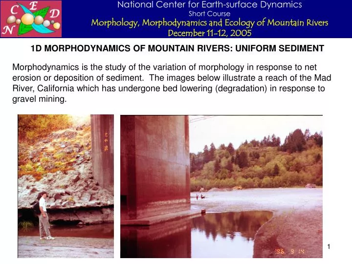
1D MORPHODYNAMICS OF MOUNTAIN RIVERS: UNIFORM SEDIMENT Morphodynamics is the study of the variation of morphology in response to net erosion or deposition of sediment. The images below illustrate a reach of the Mad River, California which has undergone bed lowering (degradation) in response to gravel mining.
AGGRADATION AND DEGRADATION A river reach aggrades (bed elevation increases) when it is supplied more sediment than it exports. A river reach degrades (bed elevation decreases) when it exports more sediment than it is supplied. Degraded reach of the Uria River, Venezuela after the Vargas disaster, 1999. Cour. J. Lopez. The Ok Tedi in Papua New Guinea had aggraded some 5 m near this bridge in response to mine disposal.
RESPONSE OF A RIVER TO SUDDEN VERTICAL FAULTING CAUSED BY AN EARTHQUAKE View in November, 1999, shortly after the earthquake caused a sharp 3 m elevation drop at a fault. View in May, 2000 after aggradation and degradation have smoothed out the elevation drop. The above images of the Deresuyu River, Turkey, are courtesy of Patrick Lawrence and François Métivier (Lawrence, 2003)
RESPONSE OF A RIVER TO SUDDEN VERTICAL FAULTING CAUSED BY AN EARTHQUAKE contd. Inferred initial profile immediately after faulting in November, 1999 Profile in May, 2001 Upstream degradation (bed level lowering) and downstream aggradation (bed level increase) are realized as the river responds to the knickpoint created by the earthquake (Lawrence, 2003).
BEDLOAD TRANSPORT The morphodynamics of mountain rivers is controlled by the differential transport of gravel moving as bedload. Bedload particles slide, roll, or saltate just above the bed, as opposed to suspended particles, which can be wafted high in the water column by turbulence. Bedload transport of uniform 7-mm gravel in a flume is illustrated below. The video clip is from the experiments of Miguel Wong.
BELOW-CAPACITY BEDLOAD TRANSPORT The video clip is from the experiments of Phairot Chatanantavet.
EXNER EQUATION FOR THE CONSERVATION OF BED SEDIMENT In 1D morphodynamics bed elevation variation is considered in the absence of width variation, and local bed features such as bars are not specifically modeled. 1D morphodynamics describes the time variation of the longitudinal profile of river bed elevation in response to net sediment deposition or erosion. The first step in characterizing 1D morphodynamics is the derivation of the Exner (19??) equation of bed sediment conservation. The parameters defined below are used in the derivation. • qb = volume bedload transport rate per unit width [L2T-1] • s = sediment density [ML3/T] • gb = sqb = mass bedload transport rate per unit width [ML-1T-1] • = bed elevation [L] p = porosity of sediment in bed deposit [1] (volume fraction of bed sample that is holes rather than sediment: 0.25 ~ 0.55 for noncohesive material) x = streamwise coordinate [L] t = time [T] B = channel width [L]
CONSERVATION OF BED SEDIMENT /t(gravel mass in control volume of bed) = mass gravel inflow rate – mass gravel outflow rate or thus This corresponds to the original form derived by Exner. The control volume has a unit width normal to x
BACKGROUND AND ASSUMPTIONS FOR 1D MORPHODYNAMICS • Change in channel bed level (aggradation or degradation) can occur in response to: • increase or decrease in upstream sediment supply; • change in hydrologic regime (water diversion or climate change); • change in river slope (e.g. channel straightening); • increased or decreased sediment supply from tributaries; • sudden inputs of sediment from debris flows or landslides; • faulting due to earthquakes or other tectonic effects such as tilting along the reach, • and; • changing base level at the downstream end of the reach of interest. Here “base level” loosely means a controlling elevation at the downstream end of the reach of interest. It means water surface elevation if the river flows into a lake or the ocean, or a downstream bed elevation controlled by e.g. tectonic uplift or subsidence at a point where the river is not flowing into standing water. Base level of this reach of the Eau Claire river, Wisconsin, USA is controlled by a reservoir, Lake Altoona
THE EQUILIBRIUM STATE contd. Rivers are different in many ways from laboratory flumes. It nevertheless helps to conceptualize rivers in terms of a long, straight, wide, rectangular flume with high sidewalls (no floodplain), constant width and a bed covered with alluvium. Such a “river” has a simple mobile-bed equilibrium (graded) state at which flow depth H, bed slope S, water discharge per unit width qw and bed material load per unit width qt remain constant in time t and in the streamwise direction x. A recirculating flume (with both water and sediment recirculated) at equilibrium is illustrated below.
THE EQUILIBRIUM STATE contd. The hydraulics of the equilibrium state are those of normal flow. Here the case of a plane bed (no bedforms) is considered as an example. The bed consists of uniform material with size D. The governing equations are (see lecture on hydraulics): Momentum conservation: Water conservation: Friction relations: where kc is a composite bed roughness which may include the effect of bedforms (if present). Generic transport relation of the form of Meyer-Peter and Müller for total bed material load: where t and nt are dimensionless constants:
THE EQUILIBRIUM STATE contd. In the case of the Chezy resistance relation, the equations governing the normal state reduce to (Slide 26 of the lecture on hydraulics): In the case of the Manning-Stickler resistance relation with an exponent of 1/6, the equations governing the normal state reduce to (Slide 30 of the lecture on hydraulics, with kc ks andg r): Let D, ks and R be given. In either case above, there are two equations for four parameters at equilibrium; water discharge per unit width qw, volume sediment discharge per unit width qt, bed slope S and flow depth H. If any two of the set (qw, qb, S and H) are specified, the other two can be computed. In a sediment-feed flume, qw and qb are set, and equilibrium S and H can be computed from either of the above pair. In a recirculating flume, qw and H are set (total water mass in flume is conserved), and qb and S can be computed.
SIMPLIFICATIONS • The concepts of aggradation and degradation are best illustrated by using simplified relations for hydraulic resistance and sediment transport. Here the following simplifications are made in addition to the assumptions of constant width and the absence of a floodplain: • The case of a Manning-Strickler formulation with constant roughness ks is considered; • Bed material is taken to be uniform with size D; • Only the portion of boundary shear stress due to skin friction is available to transport sediment; • The Exner equation of sediment conservation is based on a computation of bedload, which is computed via the generic equation • where s 1 is a constant to convert total boundary shear stress to that due to skin friction (if necessary). For example, to recover the corrected version of Meyer-Peter and Müller (1948) relation of Wong (2003) gravel transport, set t = 3.97 , nt = 1.5, c* = 0.0495 and s = 1. A setting s = 0.75 implies that 75% • of the total resistance is skin friction and 25% is form drag.
SIMPLIFICATIONS contd. 5. The full flood hydrograph or flow duration curve of discharge variation is replaced by a flood intermittency factor If, so that the river is assumed to be at low flow (and not transporting significant amounts of sediment) for time fraction 1 – If, and is in flood at constant discharge Q, and thus constant discharge per unit width qw = Q/B for time fraction If (Paola et al., 1992). The implied hydrograph takes the conceptual form below: In the long term, then, the relation between actual time t and time that the river has been in flood tf is given as Let the value of the bed material load at flood flow qb be computed in m2/s. Then the total mean annual sediment load Gt in million tons per year is given as
AN ISSUE OF NOTATION A numerical method and program for computing the 1D morphodynamics of rivers using the normal flow approximation is introduced in the succeeding slides. The code was originally written for a generic river (gravel-bed or sand-bed), for which the total volume bed material load per unit width is denoted as qt. Here this code is applied to mountain rivers, so wherever qt appears, the user of this lecture material should make the transformation
AGGRADATION AND DEGRADATION AS TRANSIENT RESPONSES TO IMPOSED DISEQIUILBRIUM CONDITIONS Aggradation or degradation of a river reach can be considered to be a response to disequilibrium conditions, by which the river tries to reach a new equilibrium. For example, if a river reach has attained an equilibrium with a given sediment supply from upstream, and that sediment supply is suddenly increased at t = 0, the river can be expected to aggrade toward a new equilibrium.
NORMAL FLOW FORMULATION OF MORPHODYNAMICS: GOVERNING EQUATIONS In this chapter the flow is calculated by approximating it with the normal flow formulation, even if the profile itself is in disequilibrium. The approximation is of loose validity in most cases of interest. It is particularly justifiable in the case of mountain rivers, as shown in the lecture on hydraulics Using the Exner formulation for sediment conservation and the Manning-Strickler formulation for flow resistance, the morphodynamic problem has the following character: In the above relations t denotes real time (as opposed to flood time) and the intermittency factor If accounts for the fact that the river is only occasionally in flood (and thus morphologically active).
THE NORMAL FLOW MORPHODYNAMIC FORMULATION AS A NONLINEAR DIFFUSION PROBLEM The previous formulation can be rewritten as: where d is a kinematic “diffusivity” of sediment (dimensions of L2/T) given by the relation The top equation is a (nonlinear) diffusion equation. In the bottom equation, it is seen that d is dependent on S = - /x, so that the diffusion formulation is nonlinear. The problem is second-order in x and first order in t, so that one initial condition and two boundary conditions are required for solution.
INITIAL AND BOUNDARY CONDITIONS The reach over which morphodynamic evolution is to be described must have a finite length L. Here it extends from x = 0 to x = L. The initial condition is that of a specified bed profile; The simplest example of this is a profile with specified initial downstream elevation Id at x = L and constant initial slope SI; The upstream boundary condition can be specified in terms of given sediment supply, or feed rate qtf, which may vary in time; The simplest case is that of a constant value of sediment feed. The downstream boundary condition can be one of prescribed base level in terms of bed elevation; Again the simplest case is a constant value, e.g. d = 0.
NOTES ON THE DOWNSTREAM BOUNDARY CONDITION • In principle the best place to locate the downstream boundary condition is at a bedrock exposure, as illustrated below. In most alluvial streams, however, such points may not be available. Three alternatives are possible: • Set the boundary condition at a point so far downstream that no effect of e.g. changed sediment feed rate is felt during the time span of interest; • Set the boundary condition where the river joins a much larger river; or • Set the boundary condition at a point of known water surface elevation, such as a lake. Alluvial Kaiya River, Papua New Guinea, and downstream bedrock exposure Bedrock makes a good downstream b.c.
Feed sediment here! DISCRETIZATION FOR NUMERICAL SOLUTION The morphodynamic problem is nonlinear and requires a numerical solution. This may be done by dividing the domain from x = 0 to x = L into M subreaches bounded by M + 1 nodes. The step length x is then given as L/M. Sediment is fed in at an extra “ghost” node one step upstream of the first node. Bed slope can be computed by the relations to the right. Once the slope Si is computed the sediment transport rate qt,i can be computed at every node. At the ghost node, qt,g = qtf.
DISCRETIZATION OF THE EXNER EQUATION Let t denote the time step. Then the Exner equation discretizes to where and au is an upwinding coefficient. In a pure upwinding scheme, au = 1. In a central difference scheme, au = 0.5. A central difference scheme generally works well when the normal flow formulation is used. At the ghost node, qt,g = qtf. In computing qt,i/x at i = 1, the node at i – 1 (= 0) is the ghost node. At node M+1, the Exner equation is not implemented because bed elevation is specified as M+1 = d.
INTRODUCTION TORTe-bookAgDegNormal.xls The basic program in Visual Basic for Applications is contained in Module 1, and is run from worksheet “Calculator”. The program is designed to compute a) an ambient mobile-bed equilibrium, and b) the response of a reach to changed sediment input rate at the upstream end of the reach starting from t = 0. The first set of required input includes: flood discharge Q, intermittency If, channel (bankfull) width B, grain size D, bed porosity p, composite roughness height kc and ambient bed slope S (before increase in sediment supply). Here composite roughness height is meant to include the effect of bedforms. For mountain streams in the absence of form drag, it is appropriate to set kc equal to ks = nkD, where nk is in the range 3 – 4. When form drag is present it is appropriate to increase nk to somewhat larger values (~ 5 or 6). Various parameters of the ambient flow, including the ambient annual bed material transport rate Gt in tons per year, are then computed directly on worksheet “Calculator”.
INTRODUCTION TORTe-bookAgDegNormal.xls contd. The next required input is the annual average bed material feed rate Gtf imposed after t > 0. If this is the same as the ambient rate Gt then nothing should happen; if Gtf > Gt then the bed should aggrade, and if Gtf < Gt then it should degrade. The final set of input includes the reach length L, the number of intervals M into which the reach is divided (so that x = L/M), the time step t, the upwinding coefficient au (use 0.5 for a central difference scheme), and two parameters controlling output, the number of time steps to printout Ntoprint and the number of printouts (in addition to the initial ambient state) Nprint. The downstream bed elevation d is automatically set equal to zero in the program. Auxiliary parameters, including r (coefficient in Manning-Strickler), t and nt (coefficient and exponent in load relation), c* (critical Shields stress), s (fraction of boundary shear stress that is skin friction) and R (sediment submerged specific gravity) are specified in the worksheet “Auxiliary Parameters”.
INTRODUCTION TORTe-bookAgDegNormal.xls contd. The parameter s estimating the fraction of boundary shear stress that is skin friction, should either be set equal to 1 or estimated using the techniques of Chapter 9. In any given case it will be necessary to play with the parameters M (which sets x) and t in order to obtain good results. For any given x, it is appropriate to find the largest value of t that does not lead to numerical instability. The program is executed by clicking the button “Do a Calculation” from the worksheet “Calculator”. Output for bed elevation is given in terms of numbers in worksheet “ResultsofCalc” and in terms of plots in worksheet “PlottheData” The formulation is given in more detail in the worksheet “Formulation”, which is also available as a stand-alone document, Rte-bookAgDegNormalFormul.doc.
MODULE 1 Sub Main This is the master subroutine that controls the Visual Basic program. Sub Main() Clear_Old_Output Get_Auxiliary_Data Get_Data Compute_Ambient_and_Final_Equilibria Set_Initial_Bed_and_time Send_Output j = 0 For j = 1 To Nprint For w = 1 To Ntoprint Find_Slope_and_Load Find_New_eta Next w More_Output Next j End Sub
MODULE 1 Sub Set_Initial_Bed_and_time This subroutine sets the initial ambient bed profile. Sub Set_Initial_Bed_and_time() For i = 1 To N + 1 x(i) = dx * (i - 1) eta(i) = Sa * L - Sa * dx * (i - 1) Next i time = 0 End Sub
MODULE 1 Sub Find_Slope_and_Load This subroutine computes the load at every node. Sub Find_Slope_and_Load() Dim i As Integer Dim taux As Double: Dim qstarx As Double: Dim Hx As Double Sl(1) = (eta(1) - eta(2)) / dx Sl(M + 1) = (eta(M) - eta(M + 1)) / dx For i = 2 To M Sl(i) = (eta(i - 1) - eta(i + 1)) / (2 * dx) Next i For i = 1 To M + 1 Hx = ((Qf ^ 2) * (kc ^ (1 / 3)) / (alr ^ 2) / (B ^ 2) / g / Sl(i)) ^ (3 / 10) taux = Hx * Sl(i) / Rr / D If fis * taux <= tausc Then qstarx = 0 Else qstarx = alt * (fis * taux - tausc) ^ nt End If qt(i) = ((Rr * g * D) ^ 0.5) * D * qstarx Next i End Sub
MODULE 1 Sub Find_New_eta This subroutine implements the Exner equation to find the bed one time step later. Sub Find_New_eta() Dim i As Integer Dim qtback As Double: Dim qtit As Double: Dim qtfrnt As Double: Dim qtdif As Double For i = 1 To M If i = 1 Then qtback = qqtf Else qtback = qt(i - 1) End If qtit = qt(i) qtfrnt = qt(i + 1) qtdif = au * (qtback - qtit) + (1 - au) * (qtit - qtfrnt) eta(i) = eta(i) + dt / (1 - lamp) / dx * qtdif * Inter Next i time = time + dt End Sub
A SAMPLE COMPUTATION The ambient sediment transport rate is 305,000 tons/year. At time t = 0 this is increased to 700,000 tons per year. The bed must aggrade in response.
INTERPRETATION The long profile of a river is a plot of bed elevation versus down-channel distance x. The long profile of a river is called upward concaveif slope S = -/x is decreasing in the streamwise direction; otherwise it is called upward convex. That is, a long profile is upward concave if Aggrading reaches often show transient upward concave profiles. This is because the deposition of sediment causes the sediment load to decrease in the downstream direction. The decreased load can be carried with a decreased Shields number *, and thus according to the normal-flow formulation of the present chapter, a decreased slope:
INTERPRETATION contd. The transient long profile of Slide 30 is upward concave because the river is aggrading toward a new mobile-bed equilibrium with a higher slope. Once the new equilibrium is reached, the river will have a constant slope (vanishing concavity). This process is outlined in the next slide (Slide 33), in which all the input parameters are the same as in Slide 29 except Ntoprint, which is varied so that the duration of calculation ranges from 1 year (far from final equilibrium) to 250 years (final equilibrium essentially reached). Slide 34 shows a case where the profile degrades to a new mobile-bed equilibrium. During the transient process of degradation the long profile of the bed is downward concave, or upward convex. This is because the erosion which drives degradation causes the load, and thus the slope to increase in the downstream direction. The input conditions for Slide 34 are the same as those of Slide 29, except that the sediment feed rate Gtf is dropped to 70,000 tons per year. This value is well below the ambient value of 305,000 tons per year (see Slide 29), forcing degradation and transient downward concavity. In addition, Ntoprint is varied so that the duration of calculation varies from 1 year to 250 years. Factors such as subsidence or base level rise can drive equilibrium long profiles which are upward concave.
ADJUSTING THE NUMBER M OF SPATIAL INTERVALS AND THE TIME STEP t The calculation becomes unstable, and the program crashes if the time step t is too long. The above example resulted in a crash when t was increased from the value of 0.01 years in Slide 29 to 0.05 years. The larger the value M of spatial intervals is, the smaller is the maximum value of t to avoid numerical instability. Acceptable values of M and t can be found by trial and error.
AN EXTENSION: RESPONSE OF AN ALLUVIAL RIVER TO VERTICAL FAULTING DUE TO AN EARTHQUAKE The code in RTe-bookAgDegNormal.xls represents a plain vanilla version of a formulation that is easily extended to a variety of other cases. The spreadsheet RTe-bookAgDegNormalFault.xls contains an extension of the formulation for sudden vertical faulting of the bed. The bed downstream of the point x = rfL (0 < rf < 1) is suddenly faulted downward by an amount f at time tf. The eventual smearing out of the long profile is then computed.
RESULTS OF SAMPLE CALCULATION WITH FAULTING contd. In time the fault is erased by degradation upstream and aggradation downstream, and a new mobile-bed equilibrium is reached.
REFERENCES Exner, F. M., 1920, Zur Physik der Dunen, Sitzber. Akad. Wiss Wien, Part IIa, Bd. 129 (in German). Exner, F. M., 1925, Uber die Wechselwirkung zwischen Wasser und Geschiebe in Flussen, Sitzber. Akad. Wiss Wien, Part IIa, Bd. 134 (in German). Lawrence, P., 2003, Bank Erosion and Sediment Transport in a Microscale Straight River, Ph.D. thesis, University of Paris 7 – Denis Diderot, 167 p. Meyer-Peter, E. and Müller, R., 1948, Formulas for Bed-Load Transport, Proceedings, 2nd Congress, International Association of Hydraulic Research, Stockholm: 39-64. Paola, C., Heller, P. L. & Angevine, C. L., 1992, The large-scale dynamics of grain-size variation in alluvial basins. I: Theory, Basin Research, 4, 73-90. Wong, M., 2003, Does the bedload equation of Meyer-Peter and Müller fit its own data?, Proceedings, 30th Congress, International Association of Hydraulic Research, Thessaloniki, J.F.K. Competition Volume: 73-80. For more information see Gary Parker’s e-book: 1D Morphodynamics of Rivers and Turbidity Currents http://cee.uiuc.edu/people/parkerg/morphodynamics_e-book.htm
1D CONSERVATION OF BED SEDIMENT FOR SIZE MIXTURES, BEDLOAD ONLY fi'(z', x, t) = fractions at elevation z' in ith grain size range above datum in bed [1]. Note that over all N grain size ranges: qbi(x, t) = volume bedload transport rate of sediment in the ith grain size range [L2/T] Or thus:
ACTIVE LAYER CONCEPT The active, exchange or surface layer approximation (Hirano, 1972): Sediment grains in active layer extending from - La < z’ < have a constant, finite probability per unit time of being entrained into bedload. Sediment grains below the active layer have zero probability of entrainment.
REDUCTION OF SEDIMENT CONSERVATION RELATION USING THE ACTIVE LAYER CONCEPT Fractions Fi in the active layer have no vertical structure. Fractions fi in the substrate do not vary in time. Thus where the interfacial exchange fractions fIi defined as describe how sediment is exchanged between the active, or surface layer and the substrate as the bed aggrades or degrades.
REDUCTION OF SEDIMENT CONSERVATION RELATION USING THE ACTIVE LAYER CONCEPT contd. Between and it is found that (Parker, 1991).
REDUCTION contd. The total bedload transport rate summed over all grain sizes qbT and the fraction pbi of bedload in the ith grain size range can be defined as The conservation relation can thus also be written as Summing over all grain sizes, the following equation describing the evolution of bed elevation is obtained: Between the above two relations, the following equation describing the evolution of the grain size distribution of the active layer is obtained:
EXCHANGE FRACTIONS where 0 1 (Hoey and Ferguson, 1994; Toro-Escobar et al., 1996). In the above relations Fi, pbi and fi denote fractions in the surface layer, bedload and substrate, respectively. That is: The substrate is mined as the bed degrades. A mixture of surface and bedload material is transferred to the substrate as the bed aggrades, making stratigraphy. Stratigraphy (vertical variation of the grain size distribution of the substrate) needs to be stored in memory as bed aggrades in order to compute subsequent degradation.
WHY THE CONCERN WITH SEDIMENT MIXTURES? Rivers often sort their sediment. An example is downstream fining: many rivers show a tendency for sediment to become finer in the downstream direction. bed slope elevation Long profiles showing downstream fining and gravel-sand transition in the Kinu River, Japan (Yatsu, 1955) median bed material grain size
upstream downstream WHY THE CONCERN WITH SEDIMENT MIXTURES ? contd. Downstream fining can also be studied in the laboratory by forcing aggradation of heterogeneous sediment in a flume. Downstream fining of a gravel-sand mixture at St. Anthony Falls Laboratory, University of Minnesota (Toro-Escobar et al., 2000) Many other examples of sediment sorting also motivate the study of the transport, erosion and deposition of sediment mixtures.
REFERENCES FOR CHAPTER 4 Hirano, M., 1971, On riverbed variation with armoring, Proceedings, Japan Society of Civil Engineering, 195: 55-65 (in Japanese). Hoey, T. B., and R. I. Ferguson, 1994, Numerical simulation of downstream fining by selective transport in gravel bed rivers: Model development and illustration, Water Resources Research, 30, 2251-2260. Paola, C., P. L. Heller and C. L. Angevine, 1992, The large-scale dynamics of grain-size variation in alluvial basins. I: Theory, Basin Research, 4, 73-90. Parker, G., 1991, Selective sorting and abrasion of river gravel. I: Theory, Journal of Hydraulic Engineering, 117(2): 131-149. Toro-Escobar, C. M., G. Parker and C. Paola, 1996, Transfer function for the deposition of poorly sorted gravel in response to streambed aggradation, Journal of Hydraulic Research, 34(1): 35-53. Toro-Escobar, C. M., C. Paola, G. Parker, P. R. Wilcock, and J. B. Southard, 2000, Experiments on downstream fining of gravel. II: Wide and sandy runs, Journal of Hydraulic Engineering, 126(3): 198-208. Yatsu, E., 1955, On the longitudinal profile of the graded river, Transactions, American Geophysical Union, 36: 655-663.