Download
1 / 15
150 likes | 289 Views
Single-Family Heating Energy SEEM Estimates and RBSA Data Research in Support of SEEM-Based Savings Estimates for Weatherization and HVAC Measures Single Family Homes . Heating kWh for Program-Eligible Homes.

E N D
Single-Family Heating EnergySEEM Estimates and RBSA DataResearch in Support of SEEM-Based Savings Estimates for Weatherization and HVAC Measures Single Family Homes Heating kWh for Program-Eligible Homes. How Supplemental Fuels and the Sample Filters used for SEEM Calibration Affect Electric Heating EnergySEEM Calibration SubcommitteeAug 6, 2013
Reminder: SEEM Calibration (Phase 1) • Purpose was to align SEEM heating energy with RBSA billing data. • Conclusion: Calibrated SEEM reliably estimates total heating energy for the type of homes used in the calibration. • Calibration based on homes where SEEM and RBSA can both estimate total heating energy. Three sample filters applied: • Omit homes that can’t be modeled in SEEM due to multiple foundation types, missing data, etc. • Omit homes with non-utility fuel use or equipment (since billing data doesn’t capture non-utility heat sources) • Omit homes with poor billing analysis results (billing data estimates aren’t reliable for these homes) (Gas-heated homes were not excluded from the calibration.) Single-Family RBSA Pie: 1404 Homes
SEEM Calibration: Phase 2 • Purpose is to adjust for electric heating energy in program-like homes. • Adjustments need to address: • Non-utility heating sources; • Program-permitted gas heat sources (e.g., gas fireplaces) • Other SEEM Calibration filters • To capture effects on program-like homes, the present analysis is based on RBSA homes with: • At least one permanently-installed electric heat source; • No gas, oil, etc. primary heating systems (FAF or Boiler); Note that heat stoves and fireplaces (any fuel) are allowed. Single-Family RBSA Pie: 1404 Homes
Overview • General approach is to estimate adjustment factors that account for electric heating energy differences between the SEEM calibration sample and program population(s). • A kWh consumption or savings value will ultimately be obtained as: Intent: this product should “reliably” estimate average electric heating kWh for the target population(s).
Overview (cont.) • Perennial question: What is the right level of granularity? • A single regional true-up factor? • Separate factors for different subpopulations defined by geography, program screening criteria, or other variables? • What can the data reliably support? • Some known limitations (for the record): • RBSA data is a snapshot (can’t address changes over time); • RBSA data is observational rather than experimental (lets us estimate correlation between building characteristics and heating energy—not quite the same as estimating savings caused by program-related measures);
Methodology Starting point: Easiest approach would be to calculate a single adjustment factor as a simple ratio, The problem: This captures the two groups’ differences with respect to all variables that drive heating energy (HDDs, insulation, non-utility heating energy, equipment, partial occupancy, ...). Instead, we want adjustment factor(s) to capture some variables’ effects (e.g., partial occupancy, non-utility heating energy). But other variables (e.g., heating equipment, HDDs, insulation) are specified in SEEM input. Don’t want to capture these variables’ effects (we want to control for these variables).
Methodology (cont.) • Regression lets us estimate individual variable effects (when other variables are held constant). • Staff believes current regression model (next slide)… • Makes physical sense; • Faithfully captures main patterns in the data; and • Is reasonably robust (not overly sensitive to random noise). • Model development and related technical issues described in the report. • Proposed model is “log-scale.” The y-variable is the natural log of annualized electric heating energy (from RBSA). • Today’s focus: • Regression results; • Adjustment factors derived from the regression results; • Uncertainty and limitations.
Regression Summary(Model fit to RBSA sites with permanently installed electric heating system and without non-electric central heating systemsand with Electric Heat > 0 kWh/yr) Adjusted R2 = 0.31
Interpretation • Regression coefficients in logarithmic models: Coefficient of describes elasticity means that a 1% increase in is associated with a 0.375% increase in electric heating kWh. Each indicator coefficient estimates (roughly) the factor by which electric heating kWh typically differs between houses that have the indicated characteristic and those that do not. Example: says that (all else being equal) a house that has a heat pump will average about 39% less electric heat kWh than one that does not. Based on the regression, the exact value is exp(-0.386) – 1 ≈ -0.32. • HDDs, UA, etc. can be specified in SEEM input. Want to control for (rather than capture) these characteristics’ effects in calculating adjustment factors. sq. ft., electric FAF, and heat pump variables are included in the model so that their effects are not be attributed to other (possibly correlated) variables.
Interpretation (cont.) Adjustments to Calibrated SEEM output (to obtain electric and other-fuel consumption for program homes). • Non-Utility Heating Fuels. Adjustment is based on C5 = -0.481 and rate of occurrence of high non-utility-fuel users in target population. • Gas Heat. Adjustment is based on C6 = -1.021 and rate of occurrence of high gas heat use in the target population • SEEM Billing Data Filter. Based on C7= -0.388 and percent of homes with poor billing data fits (as defined by the filter) in the target population. • SEEM Data Filter. Based on C8= 0.135 and percent of homes that fail the SEEM calibration data filter. • Electric Heat = 0 kWh/yr.This is a new adjustment, based on the filter applied prior to the regression. Adjustment based on percent of homes with 0 kWh (estimated from billing data). By default, all rates of occurrence could be taken as the rates observed among program-like RBSA homes. (E.g., 13.7% of our “program-like” RBSA sample reported high off-grid heat.) Other values may be justified with external research or more stringent eligibility requirements.
Concrete Example Step 1 – Determine Adjustment Amounts: Step 2 – Allocate kWh Savings. KWh debits due to wood and Gas, plus Electric “grid” savings
Quantifying non-electric heat (1) Interpreting “Wood” debit of 74 kWh: • Actual Meaning: Because some homes use lots of wood, the grid will actually see 74 kWh less in savings (on average). • Not the same as: Average home saves 74 kWh in wood heat (that’s about 252 kBtu). • Note: 74 kWh is average over all homes; only 13.7% of RBSA homes are heavy wood users. • These have larger debits (around 38% -- Step 1 of previous slide). For reference, 252 kBtu/0.137 ≈ 1.8 MBtu. Write ‘Ewood’ for average “Wood” heat efficiency. Then average “wood” heat savings is 252/E kBtu. For the record, the calculation was: 252/Ewood = (3.412/Ewood)×74
Quantifying non-electric heat (2) Should we calculate wood heat kBtu as a constant (e.g., 3.412/Ewood) times gross kWh? Matters because gross kWh depends on equipment type. • This path would treat wood heat as a percent of heating energy; • Alternatively, could treat wood heat as a percent of heat load. Staff prefers second option (seems closer to reality).
Quantifying non-electric heat (3) To treat wood heat as a percent of heat load, use Electric FAF as “reference” heat source. Then calculate wood MBtu savings separately for each heat source: • In E FAF application: kWh × 4.93 × 3.412 / Ewood • In HP application: kWh × 4.93 × 3.412 / Ewood × CHP • In BB application: kWh × 4.93 × 3.412 / Ewood × CBB Similar calculations apply to Gas Therm Savings.