Download
1 / 10
150 likes | 707 Views
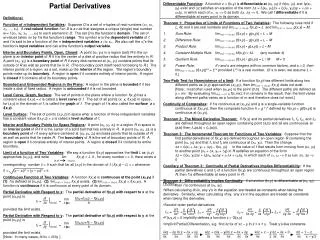
Section 14.7 Second-Order Partial Derivatives. Old Stuff. Let y = f ( x ), then Now the first derivative (at a point) gives us the slope of the tangent, the instantaneous rate of change, and whether or not a function is increasing What does the second derivative give us?

E N D
Old Stuff • Let y = f(x), then • Now the first derivative (at a point) gives us the slope of the tangent, the instantaneous rate of change, and whether or not a function is increasing • What does the second derivative give us? • If f’’(x) > 0 on an interval, f is concave up on that interval • If f’’(x) < 0 on an interval, f is concave down on that interval
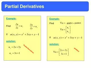
New Stuff • Suppose z = f(x,y) • Now we’ve looked at and • What do they give us? • For z we have 4 second-order partial derivatives
Let’s practice a little • Find the first and second order partial derivatives of the following functions • What do you notice about the mixed partials?
Interpretations of second order partial derivatives • If then f is concave up in the x direction or the rate of change is increasing at an increasing rate in the x direction (similar for ) • When we are looking at the mixed partials, we are looking at how a partial in one variable is changing in the direction of the other • For example, tells us how the rate of change of f in the x direction is changing as we move in the y direction
y P● 60 50 10 20 30 40 x Use the following contour plot to determine the sign of the following partial derivatives at the point, P.
We can use these in Taylor approximations • Recall we can approximate a function using a 1st degree polynomial • This polynomial is the tangent line approximation • The tangent line and the curve we are approximating have the same slope at x = a • The tangent line approximation is generally more accurate at (or around) x = a
To get a more accurate approximation we use a quadratic function instead of a linear function • In order to make this more accurate, we require that our approximation have the same value, same slope, and same second derivative at a • The Taylor Polynomial of Degree 2 approximating f(x) for x near a is
Now let z = f(x,y) have continuous first and second partial derivatives at (a,b) • Now we know from 14.3 that • Note that our approximation has the same function value and the partial derivatives have the same value as f at (a,b) • Therefore our quadratic Taylor approximation is
From we can see that our approximation matches the function value at (a,b) as well as all the partials at (a,b) • Let’s take a look at this with Maple