Download

1 / 116
1.17k likes | 1.46k Views
11. PARTIAL DERIVATIVES. PARTIAL DERIVATIVES. So far, we have dealt with the calculus of functions of a single variable. However, in the real world, physical quantities often depend on two or more variables. PARTIAL DERIVATIVES. So, in this chapter, we:

E N D
11 PARTIAL DERIVATIVES
PARTIAL DERIVATIVES • So far, we have dealt with the calculus of functions of a single variable. • However, in the real world, physical quantities often depend on two or more variables.
PARTIAL DERIVATIVES • So, in this chapter, we: • Turn our attention to functions of several variables. • Extend the basic ideas of differential calculus to such functions.
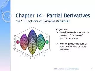
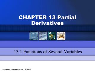
PARTIAL DERIVATIVES 11.1 Functions of Several Variables In this section, we will learn about: Functions of two or more variables and how to produce their graphs.
FUNCTIONS OF SEVERAL VARIABLES • In this section, we study functions of two or more variables from four points of view: • Verbally (a description in words) • Numerically (a table of values) • Algebraically (an explicit formula) • Visually (a graph or level curves)
FUNCTIONS OF TWO VARIABLES • The temperature T at a point on the surface of the earth at any given time depends on the longitude x and latitude y of the point. • We can think of T as being a function of the two variables x and y, or as a function of the pair (x, y). • We indicate this functional dependence by writing: T = f(x, y)
FUNCTIONS OF TWO VARIABLES • The volume V of a circular cylinder depends on its radius r and its height h. • In fact, we know that V = πr2h. • We say that V is a function of r and h. • Wewrite V(r, h) = πr2h.
FUNCTION OF TWO VARIABLES • A function f of two variables is a rule that assigns to each ordered pair of real numbers (x, y) in a set D a unique real number denoted by (x, y). • The set D is the domain of f. • Itsrange is the set of values that f takes on, that is, {f(x, y) | (x, y) D}
FUNCTIONS OF TWO VARIABLES • We often write z =f(x, y) to make explicit the value taken on by f at the general point (x, y). • The variables x and y are independent variables. • z is the dependent variable. • Compare this with the notation y =f(x) for functions of a single variable.
FUNCTIONS OF TWO VARIABLES • A function of two variables is just a function whose: • Domain is a subset of R2 • Range is a subset of R
FUNCTIONS OF TWO VARIABLES • One way of visualizing such a function is by means of an arrow diagram, where the domain D is represented as a subset of the xy-plane.
FUNCTIONS OF TWO VARIABLES • If a function f is given by a formula and no domain is specified, then the domain of fis understood to be: • The set of all pairs (x, y) for which the given expression is a well-defined real number.
FUNCTIONS OF TWO VARIABLES Example 1 • For each of the following functions, evaluate f(3, 2) and find the domain. • a. • b.
FUNCTIONS OF TWO VARIABLES Example 1 a • The expression for f makes sense if the denominator is not 0 and the quantity under the square root sign is nonnegative. • So, the domain of f is: D = {(x, y) |x +y + 1 ≥ 0, x ≠ 1}
FUNCTIONS OF TWO VARIABLES Example 1 a • The inequality x + y + 1 ≥ 0, or y ≥ –x – 1, describes the points that lie on or above the line y = –x – 1 • x ≠ 1 means that the points on the line x = 1 must be excluded from the domain.
FUNCTIONS OF TWO VARIABLES Example 1 b • f(3, 2) = 3 ln(22– 3) = 3 ln 1 = 0 • Since ln(y2– x) is defined only when y2– x > 0, that is, x < y2, the domain of f is: D = {(x, y)| x <y2
FUNCTIONS OF TWO VARIABLES Example 1 b • This is the set of points to the left of the parabola x = y2.
FUNCTIONS OF TWO VARIABLES • Not all functions are given by explicit formulas. • The function in the next example is described verbally and by numerical estimates of its values.
FUNCTIONS OF TWO VARIABLES Example 2 • In regions with severe winter weather, the wind-chill index is often used to describe the apparent severity of the cold. • This index W is a subjective temperature that depends on the actual temperature T and the wind speed v. • So, W is a function of T and v, and we can write: W =f(T, v)
FUNCTIONS OF TWO VARIABLES Example 2 • The following table records values of W compiled by the NOAA National Weather Service of the US and the Meteorological Service of Canada.
FUNCTIONS OF TWO VARIABLES Example 2
FUNCTIONS OF TWO VARIABLES Example 2 • For instance, the table shows that, if the temperature is –5°C and the wind speed is 50 km/h, then subjectively it would feel as cold as a temperature of about –15°C with no wind. • Therefore, f(–5, 50) = –15
FUNCTIONS OF TWO VARIABLES Example 3 • In 1928, Charles Cobb and Paul Douglas published a study in which they modeled the growth of the American economy during the period 1899–1922.
FUNCTIONS OF TWO VARIABLES Example 3 • They considered a simplified view in which production output is determined by the amount of labor involved and the amount of capital invested. • While there are many other factors affecting economic performance, their model proved to be remarkably accurate.
FUNCTIONS OF TWO VARIABLES E. g. 3—Equation 1 • The function they used to model production was of the form P(L, K) = bLαK1–α
FUNCTIONS OF TWO VARIABLES E. g. 3—Equation 1 • P(L, K) = bLαK1–α • P is the total production (monetary value of all goods produced in a year) • L is the amount of labor (total number of person-hours worked in a year) • K is the amount of capital invested (monetary worth of all machinery, equipment, and buildings)
FUNCTIONS OF TWO VARIABLES Example 3 • In Section 10.3, we will show how the form of Equation 1 follows from certain economic assumptions.
FUNCTIONS OF TWO VARIABLES Example 3 • Cobb and Douglas used economic data published by the government to obtain this table.
FUNCTIONS OF TWO VARIABLES Example 3 • They took the year 1899 as a baseline. • P, L, and K for 1899 were each assigned the value 100. • The values for other years were expressed as percentages of the 1899 figures.
FUNCTIONS OF TWO VARIABLES E. g. 3—Equation 2 • Cobb and Douglas used the method of least squares to fit the data of the tableto the function P(L, K) = 1.01L0.75K0.25 • See Exercise 75 for the details.
FUNCTIONS OF TWO VARIABLES Example 3 • Let’s use the model given by the function in Equation 2 to compute the production in the years 1910 and 1920.
FUNCTIONS OF TWO VARIABLES Example 3 • We get: • P(147, 208) = 1.01(147)0.75(208)0.25≈ 161.9 • P(194, 407) = 1.01(194)0.75(407)0.25≈ 235.8 • These are quite close to the actual values, 159 and 231.
COBB-DOUGLAS PRODN. FUNCN. Example 3 • The production function (Equation 1) has subsequently been used in many settings, ranging from individual firms to global economic questions. • It has become known as the Cobb-Douglas production function.
COBB-DOUGLAS PRODN. FUNCN. Example 3 • Its domain is: {(L, K) | L ≥ 0, K ≥ 0} • This is because L and K represent labor and capital and so are never negative.
FUNCTIONS OF TWO VARIABLES Example 4 • Find the domain and range of: • The domain of g is: D = {(x, y)| 9 – x2 – y2 ≥ 0} = {(x, y)| x2 + y2≤ 9}
FUNCTIONS OF TWO VARIABLES Example 4 • This is the disk with center (0, 0) and radius 3.
FUNCTIONS OF TWO VARIABLES Example 4 • The range of g is: • Since z is a positive square root, z ≥ 0. • Also,
FUNCTIONS OF TWO VARIABLES Example 4 • So, the range is: {z| 0 ≤z ≤ 3} = [0, 3]
GRAPHS • Another way of visualizing the behavior of a function of two variables is to consider its graph.
GRAPH • If f is a function of two variables with domain D, then the graph of f is the set of all points (x, y, z) in R3 such that z =f(x, y) and (x,y) is in D.
GRAPHS • Just as the graph of a function f of one variable is a curve C with equation y = f(x), so the graph of a function f of two variables is: • A surface S with equation z =f(x, y)
GRAPHS • We can visualize the graph S of f as lying directly above or below its domain Din the xy-plane.
GRAPHS Example 5 • Sketch the graph of the function f(x, y) = 6 – 3x – 2y • The graph of f has the equation z = 6 – 3x – 2y or 3x + 2y +z = 6 • This represents a plane.
GRAPHS Example 5 • To graph the plane, we first find the intercepts. • Putting y =z = 0 in the equation, we get x = 2 as the x-intercept. • Similarly, the y-intercept is 3 and the z-intercept is 6.
GRAPHS Example 5 • This helps us sketch the portion of the graph that lies in the first octant.
LINEAR FUNCTION • The function in Example 5 is a special case of the function • f(x, y) = ax +by +c • It is called a linear function.
LINEAR FUNCTIONS • The graph of such a function has the equation • z =ax +by +c • or • ax +by –z +c = 0 • Thus, it is a plane.
LINEAR FUNCTIONS • In much the same way that linear functions of one variable are important in single-variable calculus, we will see that: • Linear functions of two variables play a central role in multivariable calculus.
GRAPHS Example 6 • Sketch the graph of • The graph has equation
GRAPHS Example 6 • We square both sides of the equation to obtain: z2 = 9 – x2 – y2or x2 + y2 +z2 = 9 • We recognize this as an equation of the sphere with center the origin and radius 3.