Download
1 / 14
280 likes | 780 Views
Bayesian inference of normal distribution. Problem statement Objective is to estimate unknown two parameters q ={m,s 2 } of normal distribution based on observations y = {y 1 , y 2 , …}. Prior Joint pdf of non-informative prior Joint posterior distribution

E N D
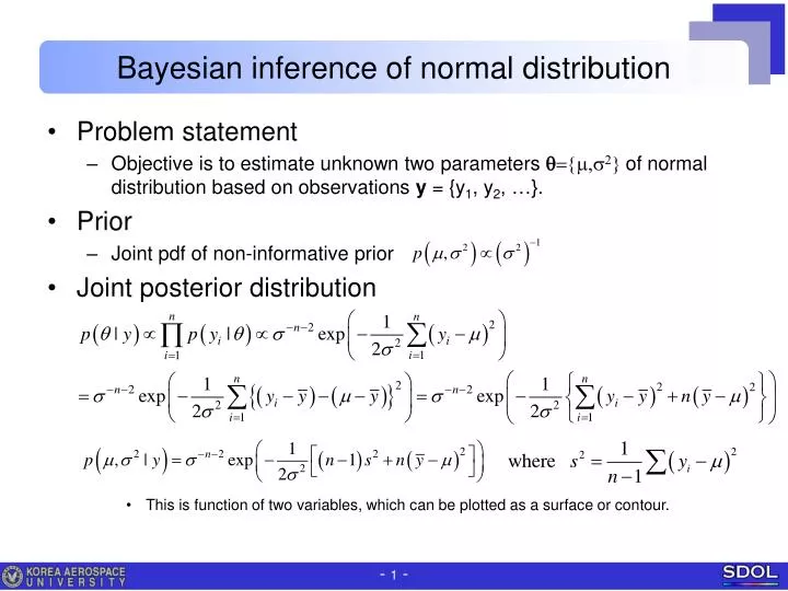
Bayesian inference of normal distribution • Problem statement • Objective is to estimate unknown two parameters q={m,s2} of normal distribution based on observations y = {y1, y2, …}. • Prior • Joint pdf of non-informative prior • Joint posterior distribution • This is function of two variables, which can be plotted as a surface or contour.
Joint posterior distribution • Distribution • There is no inherent pdf function by matlab in this case. • This is function of two variables, which can be plotted as a surface or contour. • Let’s consider a case with n=20; ȳ =2.9; s=0.2; • Remark • Analysis of posterior pdf: mean, median & confidence bounds. • Marginal distribution • Once we have the marginal pdf, we can evaluate its mean and confidence bounds. • Posterior prediction: predictive distribution of new y based on observed y. This is posterior pdf of m & s2 This is likelihood of new y
Marginal distributions • Analytical solutions • Marginal mean • Marginal variance • How to evaluate marginal distributions • Before doing this, note that in normal dist., variable y can be transformed to standard normal variable z. • Marginal mean & variance can be evaluated in the same manner. • One can evaluate various characteristics using the matlab functions.
Marginal distributions • Supplementary information for normal pdf • The original pdffY(y) and normalized pdffZ(z) have following relation. • Therefore, • If we want use f(z) instead of f(y), use this relation. • Supplementary information for chi2 pdf • The original pdffY(y) and normalized pdffZ(z) have following relation. • Therefore,
Posterior prediction • Predictive distribution of new y based on observed y • Analytical solution • One can evaluate characteristics of this using the matlab function. • Compare with the marginal mean. • Marginal mean: t-distribution with location ȳ and variance s^2/n with n-1 dof. • Predictive distribution: t-distribution with location ȳ and variance s^2*(1+1/n) with n-1 dof. posterior pdf of m & s2 Likelihood of new y
Simulation of joint posterior distribution • Why ? • Even when analytic solutions available, some are not easy to evaluate. • Once exercised, may find it more convenient and more general. • Practice simulation & validate with analytic solution. • Factorization approach • Review: joint probability of A & B • Likewise, joint posterior pdf of m & s2 • The two at the right are marginal pdfs. • Simulation by drawing random samples • We can evaluate characteristics of joint posterior pdf using simulation techniques.
Simulation of joint posterior distribution • Approach 1: use marginal variance. • Conditional pdf of m on s2 is already derived, which is the pdf of mean with known variance. (page 10 of Lec. #4) • Marginal pdf of s2 is given in this lecture. • In order to sample the posterior pdf of p(m,s2|y) • Draw s2 from the marginal pdf • Draw m from the conditional pdf Conditional pdf of m on s2 Marginal pdf of s2
Simulation of joint posterior distribution • Approach 1: use marginal variance. • Once you have obtained samples of joint pdf, compare (validate) the results with the analytic solution. • Compare the samples of (M,S2) with the analytic joint pdf. • In terms of scattered pot & contour. • In terms of 3-D histogram & surface (mesh). • Compare the samples of M with the marginal pdf, which is t distribution. • Compare the samples of S2 with the marginal pdf which is inv-chi2 distribution. • Extract features of the samples M and compare with analytic solution. • Extract features of the samples S2 and compare with analytic solution.
Simulation of joint posterior distribution • Approach 2: use marginal mean. • Conditional pdf of s2 on m is already derived, which is the pdf of variance with known mean. (page 13 of Lec. #4) • Marginal pdf of m is given in this lecture. • In order to sample the posterior pdf of p(m,s2|y) • Draw m from the marginal pdf • Draw s2 from the conditional pdf • Compare (validate) the resulting samples with the analytic solution. Conditional pdf of s2 on m Marginal pdf of m
Simulation of joint posterior distribution • Approach 2: use marginal mean. • Once you have obtained samples of joint pdf, compare (validate) the results with the analytic solution. • Details are omitted for limited time.
Posterior prediction by simulation • Analytic approach • Result of analytic solution by double integral over infinity to get • Simulation • In practice, posterior predictive distribution is obtained by random draws. • Once we have posterior distribution for m & s2 in the form of samples, the predictive new y are easily obtained by drawing each one from conditional on each individual m & s2. • Mean & conf. intervals of posterior prediction can be obtained easily.
Homework • Problems 1 • Use the approach 1 to obtain samples of joint pdf (M,S2). • Compare scattered dots with contour of analytic solution.Compare 3-D histogram with mesh shape of analytic solution. • Compare the samples of M with the marginal pdf, which is t distribution. • Compare the samples of S2 with the marginal pdf which is inv-chi2 dist. • Obtain mean, 95% conf. interval of M, & compare with analytic solution. • Obtain mean, 95% conf. interval of S2, & compare with analytic solution. • Obtain samples of posterior prediction, and obtain mean, 95% conf. interval of ynew & compare with analytic solution.