Download
1 / 17
170 likes | 181 Views
VI. Competition C. Modeling Competition 1. Intraspecific Competition 2. Interspecific Competition – Lotka-Volterra Models 3. Tilman’s Resource Models (1982). ):. 3.Tilman's Resource Models (1982). Isoclines graph population growth relative to resource ratios (2 resources, R1, R2)

E N D
VI. Competition C. Modeling Competition 1. Intraspecific Competition 2. Interspecific Competition – Lotka-Volterra Models 3. Tilman’s Resource Models (1982) ):
3.Tilman's Resource Models (1982) Isoclines graph population growth relative to resource ratios (2 resources, R1, R2) CA = Consumption rate of sp. A. ): So, species A consumes 3 units of resource 2 for every unit of resource 1.
3.Tilman's Resource Models (1982) Isoclines graph population growth relative to resource ratios (2 resources, R1, R2) CA = Consumption rate of sp. A. ): So, species A consumes 3 units of resource 2 for every unit of resource 1. BUT: It needs more resource 2; it can by on a small amount of resource 1.
3. Tilman's Resource Models (1982) Isoclines graph population growth relative to resource ratios (2 resources, R1, R2) CA = Consumption rate of Sp. A. Resource limitation can occur in different environments with different initial resource concentrations (S1, S2). So, in S2, the population becomes limited by the lower supply of R2. The lower supply of R1 in S1 is not a problem because the species uses this resource so slowly. ):
Species B requires more of both resources than species A. So, no matter the environment and no matter the consumptions curves (lines from S), the isocline for species B will be "hit" first. So, Species B will stop growing, but Species A can continue to grow and use up resources.... this drops resources below B's isocline, and B will decline.
Species B requires more of both resources than species A. So, no matter the environment and no matter the consumptions curves (lines from S), the isocline for species B will be "hit" first. So, Species B will stop growing, but Species A can continue to grow and use up resources.... this drops resources below B's isocline, and B will decline. So, if one isocline is completely within the other, then one species will always win.
If the isoclines intersect, coexistence is possible (there are densities where both species are equilibrating at values > 1).
If the isoclines intersect, coexistence is possible (there are densities where both species are equilibrating at values > 1). Whether this is a stable coexistence or not depends on the consumption curves. Consider Species B. It requires more of resource 1, but less of resource 2, than species A. Yet, it also consumes more of resource 1 than resource 2 - it is a "steep" consumption curve. So, species B will limit its own growth more than it will limit species A.
If the isoclines intersect, coexistence is possible (there are densities where both species are equilibrating at values > 1). Whether this is a stable coexistence or not depends on the consumption curves. Consider Species B. It requires more of resource 1, but less of resource 2, than species A. Yet, it also consumes more of resource 1 than resource 2 - it is a "steep" consumption curve. So, species B will limit its own growth more than it will limit species A. This will be a stable coexistence for environments with initial conditions between the consumption curves (S3). If the consumption curves were reversed, there would be an unstable coexistence in this region.
3. Tilman's Resource Models (1982) - Benefits: 1. The competition for resources is defined
3. Tilman's Resource Models (1982) - Benefits: 1. The competition for resources is defined 2. The model has been tested in plants and plankton and confirmed
3. Tilman's Resource Models (1982) - Benefits: 1. The competition for resources is defined 2. The model has been tested in plankton and confirmed Cyclotella wins Cyclotella Stable Coexistence Asterionella wins PO4 (uM) Asterionella SiO2 (uM)
3. Tilman's Resource Models (1982) - Benefits: 1. The competition for resources is defined 2. The model has been tested in plants and plankton and confirmed 3. Also explains an unusual pattern called the "paradox of enrichment"
3. Tilman's Resource Models (1982) - Benefits: 1. The competition for resources is defined 2. The model has been tested in plants and plankton and confirmed 3. Also explains an unusual pattern called the "paradox of enrichment" If you add nutrients, sometimes the diversity in a system drops... and one species comes to dominate. (Fertilize your lawn so that grasses will dominate... huh?)
If you add nutrients, sometimes the diversity in a system drops... and one species comes to dominate. Change from an initial stable coexistence scenario (S1) to a scenario where species A dominates (S2).