Download
1 / 22
220 likes | 401 Views
Earthquake Information. Summary:. Credit EMSC. Page created by W. G. Huang. Earthquake Parameters. 20100112 Haiti earthquake. Taiwan. 20090528. 20041115. 20070815. 20071114. 201002270634 Mw=8.8 D=30km. 19600522. Credit EMSC. Page created by W. G. Huang. 全球的岩石圈之主要大板塊

E N D
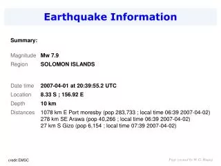
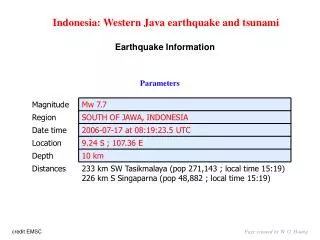
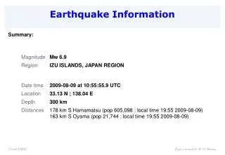
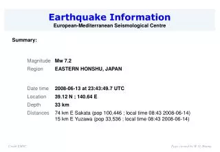
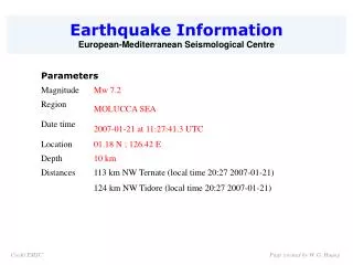
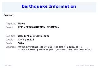
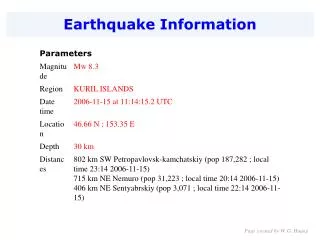
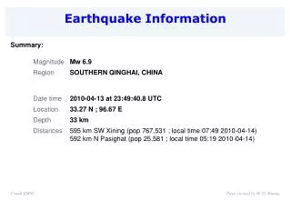
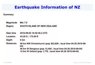
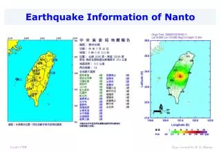
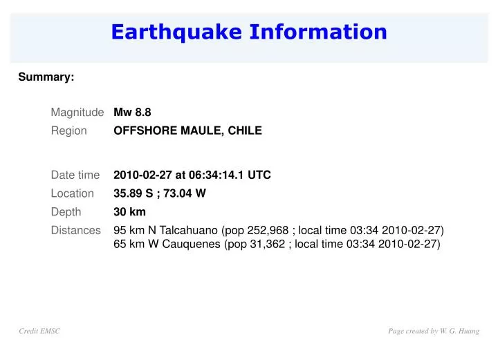
Earthquake Information Summary: Credit EMSC Page created by W. G. Huang
Earthquake Parameters 20100112 Haiti earthquake Taiwan 20090528 20041115 20070815 20071114 201002270634 Mw=8.8 D=30km 19600522 Credit EMSC Page created by W. G. Huang
全球的岩石圈之主要大板塊 MAJOR TECTONIC PLATES OF THE WORLD 歐亞板塊 Eurasian 北美板塊 North American 加勒比海板塊 Caribbean 菲律賓板塊 Philippines 太平洋板塊 Pacific 太平洋板塊 Pacific 非洲板塊 African 南美板塊 South American 印度-澳洲板塊 Indian/Australian 南極板塊 Antarctica 納薩卡板塊 Nazca Chile, like much of the west coast of South America, lies above an area of intense seismic activity and is no stranger to earthquakes. The nearby Nazca tectonic plate, which lies under the Pacific Ocean, is forced underneath the South American continental plate at a rate of about 4 cm a year. That may not sound a lot but it is enough to put huge strain on the earth's crust. The pressures are periodically released through earthquakes. Page created by W. G. Huang
20071114 Mw=7.7 20041115 Nazca Plate 20070815 20100227 Mw=8.8 20071114 19600522 M=9.5 201002270634 Mw=8.8 D=30km 19600522 M=9.5
Haze Over Santiao Following 8.8 Earthquake Credit NASA Page created by W. G. Huang
Tsunami Generation: This animation by Prof. Miho Aoki from the University of Alaska Fairbanks Art Department provides a very nice look at how a tsunami can be generated by a subduction zone earthquake.
Credit NOAA Page created by W. G. Huang
The 1960 Chilean tsunami radiated outward from a subduction zone along the coast of Chile. Its waves reached Hawaii in 15 hours and Japan in 22 hours. Credit USGS Page created by W. G. Huang
Tsunami Maximum Amplitude Plot The magnitude 8.8 earthquake in Chile on Feb. 27, 2010 The magnitude 9.5 earthquake in Chile on May 22, 1960
Fast teleseismic body-wave source inversion Martin Vallée (Géoazur, IRD, Nice, France, vallee@geoazur.unice.fr)Jean Charléty (Géoazur, CNRS, Nice, France, charlety@geoazur.unice.fr)Collaboration with A. Ferreira (UEA, Norwich,UK) and LDG/CEA (Paris, France) Method We have deconvolved the compressive (P, PcP, PP) and transverse (SH,ScS) teleseismic waves recorded by FDSN-Geoscope stations to simultaneously retrieve the focal mechanism, moment magnitude and source time functions (Frequency band : 0.005Hz -0.17Hz). Credit EMSC Page created by W. G. Huang
Source parameters, uncertainties and agreement with teleseismic data. (Top left) Optimal values of moment magnitude, depth and focal mechanism. (Bottom left) Uncertainty analysis used to determine the acceptable values of dip, depth and magnitude (see values in the bottom). (Right) Agreement between data (black) and synthetics (red), both for compressive (i.e. P, PcP, PP) waves and transverse (i.e. S, ScS) waves (frequency band : 0.005-0.03Hz). Name of the station, azimuth, distance and maximum amplitude (in microns) are shown for each signal. Credit EMSC Page created by W. G. Huang
Broadband Source time functions (RSTFs), in the time and frequency domains. (Top left) Optimal values of moment magnitude, depth and focal mechanism. (Bottom left) Spectrum of the compressive RSTFs. The classical omega-2 slope is shown in the left part of the figure. (Right) Broadband RSTFs, in the time domain, for compressive waves. For each RSTF, the name of the station, its azimuth and epicentral distance are shown Credit EMSC Page created by W. G. Huang
Finite Fault Model Preliminary Result of the Feb 27, 2010 Mw 8.8 Maule, Chile Earthquake Gavin Hayes, NEIC DATA Process and Inversion We used the GSN broadband waveforms downloaded from the NEIC waveform server. We analyzed 19 teleseismic broadband P waveforms, 8 broadband SH waveforms, and 32 long period surface waves selected based upon data quality and azimuthal distribution. Waveforms are first converted to displacement by removing the instrument response and then used to constrain the slip history based on a finite fault inverse algorithm (Ji et al, 2002). We use the hypocenter of the USGS (Lon.=-35.83 deg.; Lat.=-72.67 deg.). The fault planes are defined using the W-phase moment tensor solution of the NEIC. Credit USGS Page created by W. G. Huang
Cross-section of slip distribution Cross-section of slip distribution Cross-section of slip distribution. The strike direction of fault plane is indicated by the black arrow and the hypocenter location is denoted by the red star. The slip amplitude are showed in color and motion direction of the hanging wall relative to the footwall is indicated by white arrows. Contours show the rupture initiation time in seconds. Credit USGS Page created by W. G. Huang
Moment Rate Function Source time function, describing the rate of moment release with time after earthquake origin. Credit USGS Page created by W. G. Huang
Comparison of teleseismic body waves. The data is shown in black and the synthetic seismograms are plotted in red. Both data and synthetic seismograms are aligned on the P or SH arrivals. The number at the end of each trace is the peak amplitude of the observation in micro-meter. The number above the beginning of each trace is the source azimuth and below is the epicentral distance. Credit USGS Page created by W. G. Huang
Comparison of long period surface waves. The data is shown in black and the synthetic seismograms are plotted in red. Both data and synthetic seismograms are aligned on the P or SH arrivals. The number at the end of each trace is the peak amplitude of the observation in micro-meter. The number above the beginning of each trace is the source azimuth and below is the epicentral distance. Credit USGS Page created by W. G. Huang
Surface projection of the slip distribution superimposed on ETOPO2. The black line indicates the major plate boundary [Bird, 2003]. Credit USGS Page created by W. G. Huang
The Chilean president, Michelle Bachelet, looks down at damaged houses in Concepcion Credit Guardian Limitted Page created by W. G. Huang
Residents gather their belongings near a fishing boat washed ashore by a wave in Talcahuano Port Credit Guardian Limitted Page created by W. G. Huang
Broadband downhole seismic array in Taipei Basin Page created by W. G. Huang
The particle velocities recorded at 101B at level -100 meters.