Download
1 / 34
350 likes | 503 Views
Basic MIPS Architecture: Multi-Cycle Datapath and Control. Dr. Iyad F. Jafar. Outline. Introduction Multi-cycle Datapath Multi-cycle Control Performance Evaluation. Introduction. The single-cycle datapath is straightforward, but... Hardware duplication

E N D
Basic MIPS Architecture:Multi-Cycle Datapath and Control Dr. Iyad F. Jafar
Outline • Introduction • Multi-cycle Datapath • Multi-cycle Control • Performance Evaluation
Introduction • The single-cycle datapath is straightforward, but... • Hardware duplication • It has to use one ALU and two 32-bit adders • It has separate Instruction and Data memories • Cycle time is determined by worst-case path! Time is wasted for instructions that finish earlier!! • Can we do any better? • Break the instruction execution into steps • Each step finishes in one shorter cycle • Since instructions differ in number of steps, so will the number of cycles! Thus, time is different! • Multi-Cycle implementation!
Multi-Cycle Datapath • Instruction execution is done over multiple steps such that • Each step takes one cycle • The amount of work done per cycle is balanced • Restrict each cycle to use one major functional unit • Expected benefits • Time to execute different instructions will be different (Better Performance!) • The cycle time is smaller (faster clock rate!) • Allows functional units to be used more than once per instruction as long as they are used in different cycles • One memory is needed! • One ALU is needed!
Multi-Cycle Datapath • Requirements • Keep in mind that we have one ALU, Memory, and PC • Thus, • Add/expandmultiplexors at the inputs of major units that are used differently across instructions • Addintermediate registers to hold values between cycles !! • Defineadditional control signals and redesign the control unit
Multi-Cycle Datapath • Requirements - ALU • Operations • Compute PC+4 • Compute the Branch Address • Compare two registers • Perform ALU operations • Compute memory address • Thus, the first ALU input could be • R[rs] (R-type) • PC (PC = PC + 4) Add a MUX and define the ALUScrA signal • The second ALU input could be • R[rt] (R-type) • A constant value of 4 (to compute PC + 4) • Sign-extended immediate (to compute address of LW and SW) • Sign-extended immediate x 4 (compute branch address for BEQ) • Expand the MUX at the second ALU input and make the ALUSrcB signal two bits • The values read from register file will be used in the next cycle Add the A and B registers • The ALU result (R-type result or memory address) will be used in the following cycle Add the ALUOut register
Multi-Cycle Datapath • Requirements - PC • PC input could be • PC + 4 (sequential execution) • Branch address • Jump address The PCSrc signal • The PC is not written on every cycle • Define the PCWritesingal(for ALU, Jump, and Memory) • The PCWriteCondsingal(BEQ)
Multi-Cycle Datapath • Requirements – Memory • Memory input could be • Memory address from PC • Memory address from ALU Add MUX at the address port of the memory and define the IorD signal • Memory output could be • Instruction • Data • Add the IR register to hold the instruction • Add the MDR register to hold the data loaded from memory (Load) • The IR is not written on every cycle • Define the IRWrite signal
Multi-Cycle Datapath PCWriteCond PCWrite PCSource IorD ALUOp Control MemRead ALUSrcB MemWrite ALUSrcA MemtoReg RegWrite IRWrite RegDst 4 PC[31-28] opcode 26 28 Shift left 2 Address Field 2 0 1 Address Memory rs 0 PC Read Addr1 0 A IR Read Data 1 rt 1 Read Addr 2 zero 1 Read Data Register File 0 ALU ALUOut Write Addr rd Write Data 1 Read Data 2 B 0 Write Data 1 4 1 MDR 0 2 Sign Extend 3 Shift left 2 Offset 32 ALU control func 32
Fetch Execute Memory WB Instruction Execution • The execution of instructions is broken into multiple cycles • In each cycle, only one major unit is allowed to be used • The major units are • The ALU • The Memory • The Register File • Keep in mind that not all instructions use all the major functional units • In general we may need up to five cycles Cycle 1 Cycle 2 Cycle 3 Cycle 4 Cycle 5 Decode
Instruction Execution • Cycle 1 – Fetch • Same for all instructions • Operations • Send the PC to fetch instruction from memory and store in IR IR Mem[PC] • Update the PC PC PC + 4 • Control Signals • IorD = 0 (Select the PC as an address) • MemRead = 1 (Reading from memory) • IRWrite = 1 (Update PC) • ALUSrcA = 0 (Select PC as first input to ALU) • ALUSrcB = 01 (Select 4 as second input to ALU) • ALUOp = 00 (Addition) • PCWrite = 1(Update PC) • PCSrc = 00 (Select PC+4)
Instruction Execution • Cycle 2 – Decode • Operations • Read two registers based on the rs and rt fields and store them in the A and B registers A Reg[IR[25:21] ] B Reg[IR[20:16]] • Use the ALU to compute the branch address ALUOut PC + (sign-extend(IR[15:0]) <<2) • Is it always a branch instruction??? • Control Signals • ALUSrcA = 0 (Select PC+4) • ALUSrcB = 11 (Select the sign-extended offsetx4) • ALUOp = 00 (Add operation)
Instruction Execution • Cycle 3 – Execute & Branch and Jump Completion • The instruction is known! • Different operations depending on the instruction • Operations • Memory Access Instructions (Load or Store) • Use the ALU to compute the memory address ALUOut A + sign-extend(IR[15:0]) • Control Signals • ALUSrcA = 1 (Select A register) • ALUSrcB = 10 (Select the sign-extended offset) • ALUOp = 00 (Addition operation)
Instruction Execution • Cycle 3 – Execute & Branch and Jump Completion • Operations • ALU instructions • Perform the ALU operation according to the ALUop and Func between registers A and B ALUOut A op B • Control Signals • ALUSrcA = 1 (Select A register) • ALUSrcB = 00 (Select B register) • ALUOp = 10 (ALUoperation)
Instruction Execution • Cycle 3 – Execute & Branch and Jump Completion • Operations • Branch Equal Instruction • Compare the two registers if (A == B) then PC ALUOut • Control Signals • ALUSrcA = 1 (Select A register) • ALUSrcB = 00 (Select B register) • ALUOp = 01 (Subtract) • PCWriteCond = 1 (Branch instruction) • PCSrc = 01 (Select branch address)
Instruction Execution • Cycle 3 – Execute & Branch and Jump Completion • Operations • Jump Instruction • Generate the jump address PC {PC[31:28], (IR[25:0],2’b00)} • Control Signals • PCSrc = 10 (Select jump address) • PCWrite = 1 (Write the PC)
Instruction Execution • Cycle 4 – Memory Read or R-type and Store Completion • Different operations depending on the instruction • Operations • Load instruction • Use the computed address (found in ALUOut) , read from memory and store value in MDR MDR Memory[ALUOut] • Control Signals • IorD = 1 (Address is for data) • MemRead = 1 (Read from memory) • Store instruction • Use the computed address to store the value in register B into memory Memory[ALUOut] B • Control Signals • IorD = 1 (Address is for data) • MemWrite = 1 (Write to memory)
Instruction Execution • Cycle 4 – Memory Read or R-type and Store Completion • Operations • ALU instructions • Write the results (ALUOut) into the register filer Reg[IR[15:11]] ALUOut • Control Signals • MemToReg = 0 (Data is from ALUOut) • RegDest = 1 (Destination is rd) • RegWrite = 1 (Write to register)
Instruction Execution • Cycle 5 – Memory Read Completion • Needed for Load instructions only • Operations • ALU instructions • Store the value loaded from memory and found in the MDR register in the register file based on the rt field of the instruction Reg[IR[20:16]] MDR • Control Signals • MemToReg = 1 (Data is from MDR) • RegDest = 0 (Destination is rt) • RegWrite = 1 (Write to register)
Instruction Execution • In the proposed multi-cycle implementation, we may need up to five cycles to execute the supported instructions
Datapath control points Combinational control logic State Reg Next State Inst Opcode Multi-Cycle Control (1) FSM Implementation • The control of single-cycle is simple! All control signals are generated in the same cycle! • However, this is not true for the multi-cycle approach: • The instruction execution is broken to multiple cycles • Generating control signals is not determined by the opcode only! It depends on the current cycle as well! • In order to determine what to do in the next cycle, we need to know what was done in the previous cycle! • Memorize ! Finite state machine (Sequential circuit)! • FSM • A set of states (current state stored in State Register) • Next state function (determined by current state and the input) • Output function (determined by current state and the input) . . . . . . . . .
Multi-Cycle Control • Need to build the state diagram • Add a state whenever different operations are to be performed • For the supported instructions, we need 10 different states (next slide) • The first two states are the same for all instructions • Once the state diagram is obtained, build the state table, derive combinational logic responsible for computing next state and outputs
Multi-cycle State Diagram (9) Branch Completion (8) Jump Completion ALUSrcA = 1 ALUSrcB = 00 ALUOp = 01 PCWriteCond = 1 PCSrc = 01 PCWrite = 1 PCSrc = 10 (0) Fetch Op = J (7) R-Type Completion (6) Execute Op = BEQ (1) Decode MemRead = 1 ALUSrcA = 0 IorD = 0 IRWrite = 1 ALUSrcB = 01 ALUOp = 00 PCWrite = 1 PCSrc = 00 ALUSrcA = 0 ALUSrcB = 11 ALUOp = 00 ALUSrcA = 1 ALUSrcB = 00 ALUOp = 10 RegDst = 1 RegWrite = 1 MemtoReg = 0 START Op = R-type (5) SW Completion Op = LW Op = SW MemWrite = 1 IorD = 1 (2) Memory Address Computation Op = SW ALUSrcA = 1 ALUSrcB = 10 ALUOp = 00 (3) Memory Access (4) LW Completion Op = LW RegDst = 0 RegWrite = 1 MemtoReg = 1 MemRead = 1 IorD = 1
Multi-Cycle Control PCWrite 210x20 ROM Control Logic PCWriteCond IorD (2) ROM Implementation • FSM design • 10 inputs • 20 outputs • TT size = 210x20 • ROM • Can be used to implement the truth table above • Each location stores the control signals values and the next state • Each location is addressable by the opcode and next state value MemRead MemWrite IRWrite MemToReg PCSrc ALUOp Data ALUSrcB ALUSrcA RegWrite RegDst NS3 NS2 NS1 NS0 Address Op4 Op2 S2 Op5 Op3 S3 S1 S0 Op1 Op0 Opcode State Register
Multi-Cycle Control (3) Microprogramming • ROM implementation is vulnerable to bugs and expensive especially for complex CPU. • Size increase as the number and complexity of instructions (states) increases • Use Microprogramming • Some sort of a programming language! • The next state might not be sequential • Generate the next state outside the ROM • Each state is a micro instruction and the signals are specified symbolically • Use labels for sequencing
Multi-Cycle Control PCWrite (3) Microprogramming 10x17 ROM Control Logic PCWriteCond IorD MemRead MemWrite IRWrite MemToReg Data PCSrc ALUOp ALUSrcB ALUSrcA RegWrite RegDst Address AddCtrl 1 State Address Select Logic Opcode
Multi-Cycle Control (3) Microprogramming Inside the address select logic To ROM 1 State MUX 3 2 1 0 AddCtrl 0 Dispatch ROM 2 Dispatch ROM 1 Opcode
Multi-Cycle Control (3) Microprogramming Inside the address select logic
Multi-Cycle Control (3) Microprogramming
Multi-Cycle Performance • Example 1. Compare the performance of the multi-cycle and single-cycle implementations for the SPECINT2000 program which has the following instruction mix: 25% loads, 10% stores, 11% branches, 2% jumps, 52% ALU. • TimeSC = IC x CPISC x CCSC = IC x 1 x CCSC = ICSC x CCSC • TimeMC = IC x CPIMC x CCMC CPIMC = 0.25x5 + 0.1x4 + 0.11x3 + 0.02 x 3 + 0.52 x 4 = 4.12 CCMC = 1/5 * CCSC(Is that true!!) • Speedup = TimeSC / TimeMC= 5 / 4.12 = 1.21 ! • Multi-cycle is cost effective as well, as long as the time for different processing units are balanced!
Multi-Cycle Performance Cycle 1 Cycle 2 • Single-Cycle • Multi-Cycle • This is true as long as the delay of all functional units is balanced! LW SW waste LW SW Instr
Multi-Cycle Performance • Example 2. Redo example 1 without assuming that the cycle time for multi-cycle is 1/5 that of single cycle. Assume the delay times of different units as given in the table. • TimeSC = IC x CPISC x CCSC = IC x 1 x 600= 600 IC • TimeMC = IC x CPIMC x CCMC CPIMC = 0.25x5 + 0.1x4 + 0.11x3 + 0.02 x 3 + 0.52 x 4 = 4.12 CCMC = 200 (should match the time of the slowest functional unit) TimeMC = IC x 4.12x 200 = 824 IC • Speedup = TimeSC / TimeMC = 600 / 824= 0.782 !