Download
1 / 35
350 likes | 458 Views
Last lecture summary. SOM. supervised x unsupervised regression x classification Topology? Main features? Codebook vector? Output from the neuron?. Compettive learning. BMU Scaling Which neuron gets updated? How it will be updated? Topology preservation Neighborhood.

E N D
SOM • supervised x unsupervised • regression x classification • Topology? • Main features? • Codebook vector? • Output from the neuron?
Compettive learning • BMU • Scaling • Which neuron gets updated? • How it will be updated? • Topology preservation • Neighborhood
Variable parameters • NS (neighborhood strength) • Neighborhood size • Learning rate
Multidimensional data • IRIS (attributes: sepal length, sepal widht, petal length, petal width)
Since we have class labels, we can assess the classification accuracy of the map. • So first we train the map using all 150 patterns. • And then we present input patterns individually again and note the winning neuron. • The class to which the input belongs is the class associated with this BMU codebook vector (see previous slide, Class panel). • Only the winner decides classification.
Only winner decides the classification Vers (2) – 100% accuracy Set (1) – 86% Virg (3) – 88% Overall accuracy = 91.3% Neighborhood of size 2 decides the classification Vers (2) – 100% accuracy Set (1) – 90% Virg (3) – 94% Overall accuracy = 94.7% Sandhya Samarasinghe, Neural Networks for Applied Sciences and Engineering, 2006
U-matrix • Distances between the neighboring codebook vectors can highlight different cluster regions in the map and can be a useful visualization tool • Two neurons: w1 = {w11, w21, … wn1}, w2 = {w12, w22, … wn2} • Euclidean distance between them • The average of the distance to the nearest neighbors – unified distance, U -matrix
The larger the distance between neurons, the larger (i.e., lighter color) is the U value. Large distance between this cluster (Iris versicolor) and the middle cluster (Iris setosa). Large distances between codebook vectors indicate a sharp boundary between the clusters.
The height represents the distance. 3rd row – large height = separation Other two clusters are not separated. Surface graph
Quantization error • Measure of the distance between codebook vectors and inputs. • If for input vector x the winner is wc, then distortion errore can be calculated as • Comput e for all input vectors and get average – quantization error, average map distortion error E.
Iris quantization error High distortion error indicates areas where the codebook vector is relatively far from the inputs. Such information can be used to refine the map to obtain a more uniform distortion error measure if a more faithful reproduction of the input distribution from the map is desired.
Optimization in DM f’(x) = 0 f’’(x) > 0 … minimum f’’(x) < 0 … maximum
Optimization in DM • traditional methods (exact) • e.g. gradient based methods • heuristics (approximate) • deterministic • stochastic (chance) • e.g. genetic algorithms, simulated annealing, ant colony optimization, particle swarm optimization
Optimization in DM • Applications of optimization techniques in DM are numerous. • Optimize parameters to obtain the best performance. • Optimize weights in NN • From many features, find the best (small) subset giving the best performance (feature selection). • …
http://biology.unm.edu/ccouncil/Biology_124/Images/chromosome.gifhttp://biology.unm.edu/ccouncil/Biology_124/Images/chromosome.gif Biology Inspiration • Every organism has a set of rules describing how that organism is built up from the tiny building blocks of life. These rules are encoded in genes. • Genes are connected together into long strings called chromosomes. • Genes + alleles = genotype. • Physical expression of the genotype = phenotype. locus • gene for color • of teeth • allele for blue • teeth
When two organisms mate they share their genes. The resultant offspring may end up having half the genes from one parent and half from the other. This process is called recombination (crossover). • Very occasionally a gene may be mutated. http://members.cox.net/amgough/Chromosome_recombination-01_05_04.jpg
Life on earth has evolved through the processes of natural selection, recombination and mutation. • The individuals with better traits will survive longer and produce more offsprings. • Their survivability is given by their fitness. • This continues to happen, with the individuals becoming more suited to their environment every generation. • It was this continuous improvement that inspired John Holland in 1970’s to create genetic algorithms.
GA step by step • Objective: find the maximum of the function O(x1, x2) = x12 + x22 • This function is called objective function. • And it will be use to evaluate the fitness. Adopted from Genetic Algorithms – A step by step tutorial, Max Moorkap, Barcelona, 29th November 2005
Encoding • A model parameters (x1, x2) are encoded into binary strings. • How to encode (and decode back) a real number as a binary string? • For each real valued variable x we need to know: • the domain of the variable x ϵ [xL,xU] • length of the gene k
x1ϵ [-1, 1] x2ϵ [0, 3.1] gene • c1 = (0101110011) → (01011) = -1 + 11 * 0.0645 = -0.29 • (10011) = 0 + 19 * 0.1 = 1.9 chromosome
At the start a population of N random models is generated • c1 = (0101110011) → (01011) = -1 + 11 * 0.0645 = -0.29 • (10011) = 0 + 19 * 0.1 = 1.9 • c2 = (1111010110) → (11110) = -1 + 30 * 0.0645 = 0.935 • (10110) = 0 + 22 * 0.1 = 2.2 • c3 = (1001010001) → (10010) = -1 + 18 * 0.0645 = 0.161 • (10001) = 0 + 17 * 0.1 = 1.7 • c4 = (0110100001) → (01101) = -1 + 13 * 0.0645 = -0.161 • (00001) = 0 + 1 * 0.1 = 0.1
For each member of the population calculate the value of the objective function O(x1, x2) = x12 + x22 O1 = O(-0.29, 1.9) = 3.69 O2 = O(0.935, 2.2) = 5.71 O3 = O(0.161, 1.7) = 2.92 O4 = O(-0.161, 0.1) = 0.04 phenotype genotype
Chromosome with bigger fitness has higher probability to be selected for breeding. • We will use the following formula O1 = 3.69 O2 = 5.71 O3 = 2.92 O4 = 0.04 ∑Oj = 12.36 P1 = 0.30 P2 = 0.46 P3 = 0.24 P4= 0.003
Roulette wheel p1(30%) p2 (46%) p3 (24%) P4(0.3%)
Now select two chromosomes according to roulette wheel. • Allow the same chromosome to be selected more than once for breeding. • These two chromosomes will: • cross over • mutate • Let’s say c2 = (1111010110) and c3 = (1001010001) chromosomes were selected. • With probability Pc these two chromosomes will exchange their parts at the randomly selected locus (crossover point).
Pc Pm
Pc Pm
Pc Pm
Crossover point is selected randomly. • Pc generally should be high, about 80%-95% • If the crossover is not performed, just clone two parents into new generation. • Pm should be low, about 0.5%-1% • Perform mutation on each of the two offsprings at each locus. • Very big population size usually does not improve performance of GA. • Good size: 20-30, sometimes 50-100 reported as best • Depends on size of encoded string
Repeat previous steps till the size of new population reaches N. • The new population replaces the old one. • Each cycle throught this algorithm is called generation. • Check whether termination criteria have been met. • Change in the mean fitness from generation to generation. • Preset the number of generation.
[Start] Generate random population of N chromosomes (suitable solutions for the problem) • [Fitness] Evaluate the fitness f(x) of each chromosome x in the population • [New population] Create a new population by repeating following steps until the new population is complete • [Selection] Select two parent chromosomes from a population according to their fitness (the better fitness, the bigger chance to be selected) • [Crossover] With a crossover probability cross over the parents to form a new offspring (children). If no crossover was performed, offspring is an exact copy of parents. • [Mutation] With a mutation probability mutate new offspring at each locus (position in chromosome). • [Accepting] Place new offspring in a new population • [Replace] Use new generated population for a further run of algorithm • [Test] If the end condition is satisfied, stop, and return the best solution in current population • [Loop] Go to step 2.