Download
1 / 29
290 likes | 369 Views
Last lecture summary. New stuff. Variability is measured by standard deviation Robust equivalent? Empirical rule about stdev? Percentiles? Normal distribution, standard normal distribution Sampling distribution, CLT. Variability in sample means Standard error Centrality in sample mean

E N D
Variability is measured by standard deviation • Robust equivalent? • Empirical rule about stdev? • Percentiles? • Normal distribution, standard normal distribution • Sampling distribution, CLT
Variability in sample means • Standard error • Centrality in sample mean • Mean of sample means • Confidence interval
Margin of error exactly • The basic building block of the margin of error is the standard error . • The number of stadandard errors you want to add/subtract depends on the confidence level(hladina pravděpodobnosti). • If you want to be 95% confident with your results, you add/subtract about 2 standard errors (empirical rule).
The exact mutliple of standard error you want to ± of course depends on the confidence level and is given as • Where Z-value is a value on the standard normal distribution. confidence interval for the population mean
80% 90% 1.28 1.64 95% 99% 1.96 2.58
The above formula is correct only for large (n > 30) samples. • For n < 30 you use a different distribution called t-distribution (Student’s distribution, by William Sealy Gosset)
t-distribution is basically a shorter, fatter version of the Z-distribution • you should pay a penalty for having less information, and that penalty is a distribution with fatter tails • the larger the sample size is, the more the t-distribution looks like Z-distribution • Each t-distribution is distinguished by a number called degree of freedom (d.f.). • for the sample size of n, degrees of freedom of the corresponding t-distribution is n-1
Z t20 t1 t5
t-value in the table (one-sided, one-tailed) confidence interval for the population mean (n < 30) confidence level of 95% (97.5th percentile)
Just to repeat once more, margin of error depends on • confidence level (the most common is 95%) • sample size n • as the sample size increases, the margin of error decreases • the variability of the data (i.e. on σ) • more variability increases the margin of error • Margin of error does not measure anything else than chance variation. • It doesn’t measure any bias or errors that happens during the proces. • It does not tell anything about the correctness of your data!!!
Claims • Ecstasy use in teens dropped for the first time in recent years. The one-year decline ranged from about 1/10 to nearly 1/3, depending on what grade they were in. • A 6-month-old baby sleeps an average of 14 to 15 hours a day. • The crime in our city dropped by 4% in last six months. • Average time to cook a can of Turbo-Beans is 5 minutes.
Newspapers are full of claims like these. • While many claims are backep up by solid scientific research, other claims are not. • And now we will learn how to use stat to determine if the claim is valid. • A statistical procedure designed to test a claim is called a hypothesis test. • Hypotheses can be tested about one population parameter. Or about more. • e.g. compare average home incomes of people from two cities
Hypothesis test • Every hypothesis test contains two hypotheses: • null hypothesis Ho, H0, Ho • it states that the population parameter is equal to the claimed value (Turbo-Beans - Ho: μ=5 min) • the situation everyone asumes is true until you got involved • nothing changes, nothing happens (the previous result is the same now as it was before, e.g. catalyzed reaction) • alternative hypothesis Ha, H1, Ha • alternative model you want to consider • it stands for research hypothesis (Ha: μ≠5 min, Ha: μ<5 min, Ha: μ>5 min) • You believe that Ho is true unless you evidence shows otherwise. If you have enough evidence against Ho, you reject it and accept Ha. • If Ho is rejected in favor of Ha, a statistically significant result has been found.
After you have setup hypothesis, the next step is to collect evidence and to determine, if the claim in Ho is true or not. • Take the sample and choose your statistic. • Your Ho makes a statement about what the population parameter is (e.g. μ=5 min). • So you collect data (sample), calculate the sample statistic (x) • However, your results are based only on a sample, and we know that sample results vary!
Claim: 25% of women have varicose veins • In your sample of 100 women 20% have varicose veins • The standard error is thus cca 4% • So a difference 25% − 20% = 5% represents a distance of less than 2 standard errors away from the claim. • Therefore, you accept the claim, Ho. • However, suppose your sample was based on a sample of 1,000 women. • The standard error becomes 1.2 %, and the margin of error is 2.4 %. • Now a difference of 25% − 20% = 5% is way more than 2 standard errors away from the claim. • The claim (Ho) is concluded to be false, because your data don't support it.
The number of standard errors that a statistic lies above/below the mean is the standard score. • In order to interpret your statistic, it must be converted from original units to a standard score. • The standardized version of your statistic is called test statistic. • How to get it? • Take your statistic minus the claimed value (given by Ho) • Divide by standard error of the statistic.
Thus, test statistic represents the distance between your actual sample results and the claimed population parameter, in units of standard errors. • In the case of single population mean you know that these standardized distances should have a z-distribution (large n), or t-distribution (n < 30). • So to interpret your test statistic, you can see where it stands on the z-/t-distribution.
Although you never expect a sample statistic to be exactly the same as the population value, you expect it to be close if Ho is true. • So if the distance between the claim and the sample statistic is small, in terms of standard errors, your sample isn't far from the claim and your data are telling you to stick with Ho. • As that distance becomes larger and larger, however, your data are showing less and less support for Ho. • At some point, you should reject Ho based on your evidence, and choose Ha. At what point does this happen? That’s a question, dear Watson.
If the Ho is true, 95% of the samples will result in test statistic lying roughly within 2 standard errors of the claim. • You can be more specific about your conclusion by noting exactly how far out on the standard normal distribution the test statistic falls. Reject Ho Reject Ho Accept Ho Accept Ho
68% which percentile is this? and this? 16th 84th
You do this by looking up the test statistic on the standard normal distribution (e.g. Z-distribution) and finding the probability of being at that value or beyond it (in the same direction). • The p-value(hodnota významnosti) is a measure of the strength of your evidence against Ho. • The farther out your test statistic is on the tails of the standard normal distribution, the smaller the p-value will be, and the more evidence you have against Ho.
Let’s have a look at the case of Z-value = -3.0, 0.13th percentile • if Ha contains less-than alternative, do: p-value 0.13/100 = 0.0013 (one-sided test) • if Ha contains greater-than alternative, do: p-value = (100-0.13)/100 = 0.9987 (one-sided test) • if Ha is the not-equal-to alternative, do: p-value = 2 * 0.13/100 = 0.0026 (two-sided test) • Choose the cutoff α(hladinavýznamnosti)(typically 0.05) p-value < α, reject Ho p-value > α, accept Ho
Errors in Testing • Type-1 error, Type I error • Errors occur because the conclusions are based on the sample, not on the whole population. Sample results vary from sample to sample. • If your test statistic falls on the tail of the standard normal distribution, these results are unusual (you expect them to be much closer to the middle of the Z-distribution). • But just because the results from a sample are unusual, however, doesn't mean they're impossible. • You conclude that a claim isn't true but it actually is true. • You reject Ho, while you shouldn’t. • You make false alarm. • False positive.
The chance of making a Type I error is equal to α, which is predetermined before you begin collecting your data. • To reduce the chance of Type I error, reduce α. • However, if you reduce too much, you increase a chance for Type II error • Type-2 error, Type II error • You conclude that a claim is true but it actually isn't. • You do not reject Ho, while you should. • You miss an opportunity. • False negative.
The chance making a Type II error depends mainly on the sample size. • If you have more data, you’re less likely to miss something that’s going on. • However, large sample increases the chance of Type I error. • Type I and Type II errors sit on opposite ends of a seesaw - as one goes up, the other goes down. • To try to meet in the middle, choose a large sample size and a small α level (0.05 or less) for your hypothesis test.