Download
1 / 40
400 likes | 417 Views
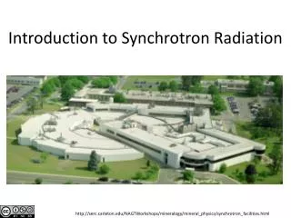
Synchrotron radiation. R. Bartolini John Adams Institute for Accelerator Science, University of Oxford and Diamond Light Source. JUAS 2017 Week 4 - 2017. Contents. Introduction to synchrotron radiation properties of synchrotron radiation synchrotron light sources

E N D
Synchrotron radiation R. Bartolini John Adams Institute for Accelerator Science, University of Oxford and Diamond Light Source JUAS 2017 Week 4 - 2017
Contents Introduction to synchrotron radiation properties of synchrotron radiation synchrotron light sources angular distribution of power radiated by accelerated particles angular and frequency distribution of energy radiated: radiation from undulators and wigglers Beam dynamics with synchrotron radiation electron beam dynamics in storage rings radiation damping and radiation excitation emittance and brilliance low emittance lattices diffraction limited storage rings short introduction to free electron lasers (FELs)
Y X-ray‘s S X Brilliance and emittance X-ray‘s As = Cross section of electron beam / = Opening angle in vert. / hor. direction Flux = Photons / ( s BW) Brilliance = Flux / ( As ) , [ Photons / ( s mm2 mrad2 BW )] The brilliance represents the number of photons per second emitted in a given bandwidth that can be refocus by a perfect optics on the unit area at the sample.
The brilliance of a storage ring based synchrotron light source can be increased by reducing the emittance of the beam, up to the limit where the natural diffraction prevents any further reduction of the photon beam size and divergence. Diffraction limit storage rings (I) This is called diffraction limited storage ring. In the expression appearing in the denominator of the brilliance the natural photon beam size ph and divergence ‘ph dominate over the size and divergence of the electron beam The condition for diffraction limit depends on the wavelength. To see this we must consider the photon beam size and divergence.
Usually the undulator radiation is approximated as the fundamental e.m. mode of a Gaussian beam. For the fundamental Gaussian mode we have ID radiation beam size (I) The Gaussain beam size and divergence of such mode are given by the relations
The undulator radiation is not striclty speaking a Gaussian mode (especially in helical undulators). However its angular distribution can be fitted with that of a Gaussian mode and the corresponding beam size and divergence are extracted from the fit: ID radiation beam size (II) The diffraction limited emittance of the photon beam of the undulator radiation generated by a filament beam is given by the product
The contribution to the photon beam size and divergence due to a finite electron beam size and divergence add in quadrature (still within the Gaussian approximation for both). The condition for diffraction limit is then given by Diffraction limit storage rings (II) The condition for diffraction limit depends on the wavelength. Usually it is quoted that of 1 Angstron (hard X rays) the emittance should be less than 8 pm (/4). The brilliance reads
Notice that the transverse emittance is minimised when the electron beam size and divergence are matched to the photon beam size and divergence, hence Diffraction limit storage rings (III) This requires a special design of the optics in the ID straight sections Courtesy B. Hettel
Reducing the emittance increseas also the transverse coherence of the radiaiton The coherent fraction is defined as the ratio of the photon flux which is diffraciton limited, hence Diffraction limit storage rings (IV) A source where the electron beam has the same size and divergence of the photon beam correspond to a coherent fraction of only 50% (in each plane!) Smaller electron beam emittances are necessary to increase the coherent fraction (beside increasing the brilliance) Courtesy B. Hettel
Emittance of third generation light sources The brilliance of the photon beam is determined (mostly) by the electron beam emittance that defines the source size and divergence. The horizontal emittance of existing light sources are very far from the diffraction limit
Emittance of third generation light sources The emittance in the vertical plane however has been reduced to the pm range in several light sources. This radiation is diffraction limited in the vertical plane up to the hard X-rays • operating • under construction
Records for smallest vertical emittance (2011-2014) SLS 0.9 pm Courtesy L. Rivkin PSI and EPFL APS 0.35 pm
Low Emittance lattices Lattice design has to provide low emittanceandadequate space in straight sections to accommodate long Insertion Devices Minimise and D and be close to a waist in the dipole Zero dispersion in the straight section was used especially in early machines avoid increasing the beam size due to energy spread hide energy fluctuation to the users allow straight section with zero dispersion to place RF and injection decouple chromatic and harmonic sextupoles DBA and TBA lattices provide low emittance with large ratio between Flexibility for optic control for apertures (injection and lifetime)
3rd generation storage ring LS and damping rings Specific lattices are used in synchrotron light sources • (FODO) • TME like lattices • DBA • TBA • QBA • MBA • controlled dispersion in straight sections Other specific techniques fare used or reducing the emittance, using • gradient dipoles • longitudinal gradient dipoles • insertion devices and damping wigglers (NSLS-II) MAX IV, Pep-X
APS ALS Low emittance lattices Low emittance and adequate space in straight sections to accommodate long Insertion Devices are obtained in Double Bend Achromat (DBA) Triple Bend Achromat (TBA) TBA used at ALS, SLS, PLS, TLS … DBA used at: ESRF, ELETTRA, APS, SPring8, Bessy-II, Diamond, SOLEIL, SPEAR3 ...
Breaking the achromatic condition Leaking dispersion in straight sections reduces the emittance ESRF 7 nm 3.8 nm APS 7.5 nm 2.5 nm SPring8 4.8 nm 3.0 nm SPEAR3 18.0 nm 9.8 nm ALS (SB) 10.5 nm 6.7 nm APS The emittance is reduced but the dispersion in the straight section increases the beam size ASP Need to make sure the effective emittance and ID effects are not made worse
Low emittance lattices MAX-IV New designs envisaged to achieve sub-nm emittance involve Damping Wigglers Petra-III: 1 nm NSLS-II: 0.5 nm MBA MAX-IV (7-BA): 0.5 nm Spring-8 (10-BA): 83 pm (2006) 10-BA had a DA –6.5 mm +9 mm reverted to a QBA (160 pm) now 6BA with 70 pm Spring-8 upgrade
Where is the equilibrium emittance generated? The formula for the emittance tells us that the emittance is generated in the dipoles (and insertion devices), i.e. in the elements where radiation is generated. In fact emittance is determined by the equilibrium between radiation diffusion and radiation damping We can try to tailor the optics functions in each single dipole in order to reduce the value of <H>dip. Indeed it is possible to show that there is a minimum emittance condition This condition can be used to generate TME-like lattice with long straight sections by using matching sections. Let us start with a single dipole…
Minimum emittance from a single dipole (I) We want the general expression for <H> dipoles in terms of the initial optics function, at the beginning of the dipole. In this way becomes a function of (0, 0, D0, D’0) since 0 will be uniquely defined by 0 and 0. The TME condition is found by setting the gradient of <H> dipoles to zero with respect to (0, 0, D0, D’0). It is often common to operate with achromatic condition in the straight section, which means fixing D0 and D’0 to zero at the entrance or at the exit of the magnet. In doing so we lose two fit parameters, since (D0, D’0) = (0, 0), and accordingly the minimum emittance value will be higher than that achieved in the general case. Let us see how the optics functions evolve in a sector bending magnet
Minimum emittance from a single dipole (II) If the dipole radius is and the gradient is K we let and naming The optics functions in the dipole evolve as and the dispersion in the sector bend reads
Minimum emittance from a single dipole (III) Using the previous equations we can compute the dispersion invariant and integrate it over the dipole length. Check this as an exercise! This expression is usually simplified in the literature. Assume that • no combined function gradient exists, i.e. K = 0 • the bend angle is small. Approximate = L/ << 1
Minimum emittance from a single dipole (IV) We now look for the initial optic functions that minimise the previous expression. Making the gradient of <H>dipole zero we obtain the following results This minimum is reached for the following set of optics functions computed at the centre of the dipoles This optics gives the theoretical minimum emittance (TME) in the limit of small dipole angle theoretical minimum emittance
Minimum emittance from a single dipole (V) The optics through the dipole looks like Courtesy A. Streun To build now a full lattice we can flank this dipole by a matching sections to create a full ring, repeating periodically the TME-cell Since 3 many small angle bending are favoured to reach smaller emittances The dispersion is non zero in the straight section and it cannot be zeroed without further dipoles
Minimum emittance from a single dipole (VI) If we start with an achromatic condition at the beginning (or end) of the dipole we must find a minimum of <H> dipoles as a function of (0, 0) with (D0, D’0) = (0, 0) The average of the dispersion invariant is this is three time larger than the TME The condition for the minimum emittance and requires that the focus of the beta function (f = 0), i.e. the minimum of is reached in the first half of the dipole and occurs at and reads In this case, the values of the optics functions at the entrance of the dipole are
Minimum emittance from a single dipole (VII) The optics through the dipole looks like Courtesy A. Streun To close the dispersion this cell can be repeated mirror symmetrically using a quadrupoles. This is the simplest from of a double bend achromat called Chashman-Green lattice Since 3 many small angle bending are favoured to reach smaller emittances
Double bend achromat A matching section can be added to tailor the optics for an insertion device as in Courtesy A. Streun This is the basic structure of a DBA lattice used in many light sources The horizontal emittance reached in medium size machines is in the order of few nm DBA theoretical minimum emittance
Triple bend achromat A TME cell can be added in between a DBA cell to generate a TBA cell Courtesy A. Streun Notice that we cannot naively assume that the minimum emittance of the TBA is the average of the TME of a DBA and one TME cell. We need to match the optics function between the two cells and this proves to be impossible if we use only quadrupoles and leave the same type of dipole, i.e. same strength and same length. In particular we cannot match the dispersion invariant at the dipole end s The condition for matching with minimum emittance require the external dipole to be shorter by 1/sqrt(3).
Low emittance with multiple bend achromats DBA 7BA Simplified explanation – Emittance is driven by randomness of photon emission in presence of dispersive (energy-dependent) orbits – electron recoils randomly – Breaking up dipoles and putting focusing (quadrupoles) between the parts allows reducing the amplitude of dispersive orbits – smaller electron recoils
Multi bend achromat In much the same way more than one TME cell can be added in between a DBA cell to generate a MBA cell With many small bending magnets the overall scaling of the emittance 3 will generate very small emittances As the Pep-X lattice a 7BA with 5 TME cells 5 TME units
Summary The formula for the emittance can be summarised as where In general we can say that the emittance scaling with the cubic power of the bending angle favours rings with a large number of bending and therefore, broadly speaking with a large circumference C.
Emittance vs circumference The design of the most recent synchrotron light sources pushes the emittance close to the diffraction limit at hard X-rays also in the horizontal plane
Further emittance reduction: damping wigglers (I) Insertion device can have a strong impact on the equilibrium beam properties, namely on the emittance The IDs modify the radiation integrals. The modification to the equilibrium beam properties can be computed from the modification to the radiation integrals (usually I4 << I2) Let us consider a insertion device made by a linear undulator with peak field BID and period u. The curvature radius associated to the trajectory reads where is the bending radius corresponding to the peak magnetic field BID of the ID.
Modification to the radiation integrals I2 and I3 The computation of the additional terms generated by the IDs requires some care. The radiation integrals depending only on the radius of curvature are straightforward where LID the length of the ID. They both increase with the ID field and ID length. The radiation integrals involving also the dispersion and the optics functions are usually calculated assuming either that the self-dispersion is negligible or, on the opposite end, that there is only the self-dispersion contribution. Let us see how to compute the self dispersion generated by the ID:
Self dispersion in IDs The ID, as any bending magnet, also modifies the dispersion function. The effect of the ID on the dispersion is usually characterised by the concept of self-dispersion, i.e. the dispersion generated by the ID in a straight section in absence of any other dispersion. The self dispersion in the ID is given by When self dispersion dominates we have The second term dominates the first, therefore we are left with
External dispersion in IDs If the external dispersion is large and self dispersion can be neglected we have The expression for I5,ID can be computed by using the value of the dispersion invariant Hi,ID at the centre of the straight section which usually has a waist for the optics function, i.e. I, ID = 0, therefore The radiation integral reads
Emittance reduction with IDs Using the modified radiation integrals we can write down the expression for the equilibrium properties of the beam in a storage ring with IDs. If I5 is dominated by external dispersion, isomagnetic lattice, we can write Thus the emittance can be increased or decreased depending on the relative values of H and r in the insertion device and in the bending magnets. If I5 is dominated by self-dispersion, in the isomagnetic case ,we have Alternatively these expression can be used to define the limits on the insertion devices field in order not to change the equilibrium properties of the beam
Example: Pep-X design Emittance = 11 pm-rad at 4.5 GeVwith parameters lw=5 cm, Bw=1.5 T Wiggler Field Optimization Wiggler Length Optimization Average beta function at the wiggler section is 12.4 meter.
Energy spread change with IDs In a similar way, using the radiation integral I2 I3, and I4 can compute the modification to the energy spread as per Since usually I4 << I2 we have In this regime, the energy spread is defined by the radiation integrals that do not depend on the dispersion function. We have the ratio If the peak field in the ID is less than that of the bending magnets (ID > ) there is a reduction in energy spread, whereas if the peak ID field exceeds the bending magnet field (ID > ) the energy spread is increased.
Small emittance Strong quadrupoles Large (natural) chromaticity Difficulties with low emittance lattices strong sextupoles (sextupoles guarantee the focussing of off-energy particles) Courtesy A. Streun strong sextupoles reduce the dynamic aperture and the Touschek lifetime additional sextupoles are required to correct nonlinear aberrations
It is a complex process where the Accelerator Physicist is guided by • (semi-)analytical formulae for the computation of nonlinear maps, detuning with amplitude and off-momentum, resonance driving terms • numerical tracking: direct calculation of non linear tuneshifts with amplitude and off-momentum, 6D dynamics aperture and the frequency analysis of the betatron oscillations Many iterations are required to achieve a good solution that guarantees a good dynamic aperture for injection and a good Touschek lifetime See lectures on nonlinear dynamics Nonlinear beam dynamics optimisation (I)