Introduction to Quantitative Analysis

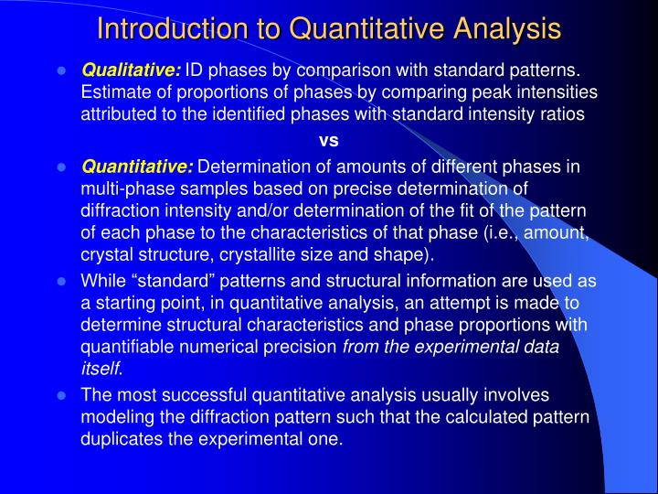
1. Introduction to Quantitative Analysis • Qualitative: ID phases by comparison with standard patterns. Estimate of proportions of phases by comparing peak intensities attributed to the identified phases with standard intensity ratios vs • Quantitative: Determination of amounts of different phases in multi-phase samples based on precise determination of diffraction intensity and/or determination of the fit of the pattern of each phase to the characteristics of that phase (i.e., amount, crystal structure, crystallite size and shape). • While “standard” patterns and structural information are used as a starting point, in quantitative analysis, an attempt is made to determine structural characteristics and phase proportions with quantifiable numerical precision from the experimental data itself. • The most successful quantitative analysis usually involves modeling the diffraction pattern such that the calculated pattern duplicates the experimental one.

2. The Intensity Equation where: • I(hkl)= Intensity of reflection of (hkl) in phase . • I0 = incident beam intensity • r = distance from specimen to detector •  = X-ray wavelength • 2nd term = square of classical electron radius • Mhkl = multiplicity of reflection hkl of phase  • Next to last term on right = Lorentz-polarization (and monochromator) correction for (hkl) • In that term, 2m = diffraction angle of the monochromator • v = volume of the unit cell of phase  • s = linear absorption coefficient of the specimen • F(hkl) = structure factor for reflection hkl of phase  (i.e., the vector sum of scattering intensities of all atoms contributing to that reflection).

3. The Intensity Equation • Recognizing that many of the terms are consistent for a particular experimental setup we can define an experimental constant, Ke. • For a given phase we define another constant, K(hkl), that is effectively equal to the structure factor term for phase . • Substituting the weight fraction (X) for the volume fraction, the density of the phase () for the volume, and the mass absorption coefficient of the specimen ( /)s for the linear absorption coefficient yields the following equation: Assuming we can get accurate intensity measurements, the big problem relates to the mass absorption coefficient for the sample, ( /)s. In most experiments ( /)s is a function of the amounts of the constituent phases and that is the object of our experiment. All peak intensity-related methods for quantitative analysis involve circumventing this problem to make this equation solvable.

4. Sample Preparation & Particle Size Issues • As discussed previously, to achieve peak intensity errors of less than 1% for a single phase (100% of specimen) requires particles between 0.5 and 1.0 m in size. • Sizes of 1-5 m are more reasonable in “real life” practice • Multi-phase specimens add to the error in inverse relation to their proportions (lower proportions = larger error) • Bottom line is reported errors of less that 5% in intensity-related multi-phase quantitative analyses are immediately suspect • Most rock specimens and many engineered materials exhibit compositional particle (i.e., crystallite) size inhomogeneities that can affect intensity measurements significantly • Following are a summary of the various factors affecting intensity measurements in diffraction:

5. Introduction to Quantitative Analysis • 1. Structure-sensitive Factors • Atomic scattering factor • Structure factor • Polarization • Multiplicity • Temperature • Most of these factors are included in the K(hkl) term in the intensity equation, and are intrinsic to the phase being determined • Temperature can affect resultant intensities • Keeping data collection conditions consistent for specimens and standards is critical for good intensity data

6. Introduction to Quantitative Analysis • 2. Instrument-sensitive Factors • (a) Absolute intensities • Source Intensity • Diffractometer efficiency • Voltage drift • Takeoff angle of tube • Receiving slit width • Axial divergence allowed • (b) Relative intensities • Divergence slit aperture • Detector dead time • Bottom line issues: • Optimize operational conditions of the diffractometer • Intensities of strongest peaks can be affected by detector dead time – apply the appropriate correction to your data

7. Introduction to Quantitative Analysis • 3. Sample-sensitive Factors • Microabsorption • Crystallite size • Degree of crystallinity • Residual stress • Degree of particle overlap • Particle orientation • All of these are discussed in the chapter on specimen preparation and related errors • Bottom line to minimize these is to keep particle (i.e., crystallite) size as close to 1m as possible

8. Introduction to Quantitative Analysis • 4. Measurement-sensitive Factors • Method of peak area measurement • Degree of peak overlap • Method of background subtraction • K2 stripping or not • Degree of data smoothing employed • Some approaches to minimizing these errors: • Be consistent in how background is removed from pattern before calculating peak areas – Accuracy of RIR-based methods depend on consistency in picking backgrounds • Always use integrated peak area for intensity • Avoid overlapping peaks or, if unavoidable, use digital peak deconvolution techniques to resolve overlapping peaks • Jade includes tools for removing background and stripping K2 peaks, peak decomposition into components, and analyzing peak shapes (for size, shape and strain analysis).

9. What is the RIR? • RIR is an intensity ratio of a peak area in a determined phase to that of a standard phase (usually corundum) • It is a ratio of the integrated intensity of the strongest peak of the phase in question to the strongest peak of corundum • I/Ic (RIRcor) is published for many phases in the ICDD PDF database • It may be experimentally determined for particular systems and used in “spiked” specimens

10. RIR depends on background picks

11. Absorption-Diffraction Method The relationship between I for phase in a specimen and I of the pure phase:Note that (/)s is unknown. In the specialized case where the absorption coefficients for the phase and specimen are identical: For the specialized case of a binary mixture where (/) is known for each phase, the relationship is described by the Klug equation: For the general case, (/)s must be estimated. This may be done if bulk chemistry is known using elemental mass attenuation coefficients.

12. Internal Standard Method A known amount of a standard (typically 10-20 wt %) is added to a specimen containing phase  to be determined. The absorption coefficient for the sample drops out of the equation yielding: For this to work the constant k must be experimentally determined using known proportions of the standard and phase in question. Standards should be chosen to avoid overlap of peaks with those in the phases to be determined Requires careful specimen preparation and experimental determination of k at varying proportions of the two phases

13. Reference Intensity Ratio Methods I/Icorundum • Rearranging the intensity equation, and plotting vs Yields a straight line with a slope k. These k values using corundum as the  phase in a 50:50 mixture are now published with many phases in the ICDD PDF database as RIRcor Theoretically the could be used as for a direct calculation of amounts (with factors to adjust for actual standard proportions) Practically, they are inaccurate because of experimental variables related to particle size and diffractometer characteristics. 1 micron corundum powder is available for use as lab standard

14. PDF#46-1045: QM=Star(+); d=Diffractometer; I=Diffractometer Quartz, syn Si O2 (White) Radiation=CuKa1 Lambda=1.5405981 Filter=Ge Calibration=Internal(Si) d-Cutoff= I/Ic(RIR)=3.41 Ref= Kern, A., Eysel, W., Mineralogisch-Petrograph. Inst., Univ. Heidelberg, Germany. ICDD Grant-in-Aid (1993) Hexagonal - Powder Diffraction, P3221(154) Z=3 mp= Cell=4.9134x5.4052 Pearson=hP9 (O2 Si) Density(c)=2.650 Density(m)=2.660 Mwt=60.08 Vol=113.01 F(30)=538.7(.0018,31) Ref= Z. Kristallogr., 198 177 (1992) Strong Line: 3.34/X 4.26/2 1.82/1 2.46/1 1.54/1 2.28/1 1.38/1 2.13/1 1.38/1 2.24/1 NOTE: Pattern taken at 23(1) C. Low temperature quartz. 2$GU determination based on profile fit method. To replace 33-1161. d(A) I(f) I(v) h k l n^2 2-Theta Theta 1/(2d) 2pi/d 4.255 16.0 13.0 1 0 0 1 20.859 10.430 0.1175 1.4767 3.343 100.0 100.0 1 0 1 2 26.639 13.320 0.1495 1.8792 2.456 9.0 12.0 1 1 0 2 36.543 18.272 0.2035 2.5574 2.281 8.0 12.0 1 0 2 5 39.464 19.732 0.2192 2.7540 2.236 4.0 6.0 1 1 1 3 40.299 20.149 0.2236 2.8098 2.127 6.0 9.0 2 0 0 4 42.449 21.224 0.2350 2.9530 1.979 4.0 7.0 2 0 1 5 45.792 22.896 0.2525 3.1736 1.818 13.0 24.0 1 1 2 6 50.138 25.069 0.2750 3.4562 1.801 1.0 2.0 0 0 3 9 50.621 25.310 0.2775 3.4873 1.671 4.0 8.0 2 0 2 8 54.873 27.437 0.2991 3.7585 1.659 2.0 4.0 1 0 3 10 55.323 27.662 0.3014 3.7869 1.608 1.0 2.0 2 1 0 5 57.234 28.617 0.3109 3.9068 1.541 9.0 20.0 2 1 1 6 59.958 29.979 0.3244 4.0759 PDF card with RIRcor Value

15. RIR Methods • I/Ic is a specialized RIR defined in terms of the 100% peak of different phases. Theoretically RIRs may be determined for any peak enabling overlapping peaks to be avoided. • A generalized RIR equation: • The Irel term ratios the relative intensities of the peaks used – if the 100% peaks are used, the value of this term is 1 • Common internal standards in use include: • -Al2O3 (corundum) • Quartz (SiO2) • ZnO

16. RIR Methods • Rearranging the Generalized RIR equation yields: Particular RIRs may be derived from other RIR values: In practice, “derived” RIRs should be avoided, and experimental RIRs carefully determined in the laboratory should be used. With good RIR values and careful sample preparation, the method can yield decent quantitative results. Because each phase is determined independently, this method is suitable for samples containing unidentified or amorphous phases.

17. Normalized RIR (Chung) Method • Chung (1974) recognized that if all phases are known and RIRs known for all phases, then the sum of all of the fractional amounts of the phases must equal 1, allowing the calculation of amounts of each phase: Chung called this the “matrix flushing” method or adiabatic principle; it is now generally called the normalized RIR (or Chung) method and allows “quantitative” calculations without an internal standard present Local experimental determination of the RIRs used can improve the quality of the results but . . . The presence of any unidentified or amorphous phases invalidates the use of the method. In virtually all rocks there will be undetectable phases and thus the method will never be rigorously applicable

18. Constrained Phase Analysis • If independent chemical information is available that constrains phase composition, this may be integrated with peak intensity and RIR data to constrain the results • The general approach to this can include normative chemical calculations, constraints on the amounts of particular phase based on limiting chemistry constraints etc. • The general approach to this type of integrated analysis is discussed by Snyder and Bish (1989)

19. Rietveld Full-Pattern Analysis • The full-pattern approach pioneered by Dr. Hugo M. Rietveld attempts to account for all of the contributions to the diffraction pattern to discern all of the component parts by means of a least-squares fit of the diffraction pattern • The method is made possible by the power of digital data processing and very complicated software • Originally conceived only for use with extremely clean neutron diffraction data, the method has evolved to deal with the relatively poor-quality of data from conventionally-sourced diffractometers • The quantity minimized in the analysis is the least squares residual: where Ij(o) and Ij(c) are the intensity observed and calculated, respectively, at the jth step in the data, and wj is the weight.

20. Rietveld Full-Pattern Analysis • The method is capable of much greater accuracy in quantifying XRD data than any peak-intensity-based method because of the systemic “whole-pattern” approach • The initial primary use of the method was (and still is) to make precise refinements of crystal structures based on fitting the experimental diffraction pattern to precise structure • As with the Normalized RIR method, all phases in the pattern must be identified and baseline structural parameters are input into the model; an internal standard is required to calibrate scale factors if there are unidentified phases present • Reitveld’s 1969 paper is recommended for further reading (linked on our class website) • Though it generally has a fairly steep learning curve, very sophisticated software is available at no cost to do the refinements: Major packages include GSAS and FullPROF

21. Rietveld Full-Pattern Analysis Advantages over other methods: • Differences between the experimental standard and the phase in the unknown are minimized. Compositionally variable phases are varied and fit by the software. • Pure-phase standards are not required for the analysis. • Overlapped lines and patterns may be used successfully. • Lattice parameters for each phase are refined by processing, allowing for the evaluation of solid solution effects in the phase. • The use of the whole pattern rather than a few select lines produces accuracy and precision much better than traditional methods. • Preferred orientation effects are averaged over all of the crystallographic directions, and may be modeled during the refinement.

22. Rietveld Full-Pattern Analysis Qualitative summary of Rietveld variables: • Peak shape function describes the shape of the diffraction peaks. It starts from a pure Gaussian shape and allows variations due to Lorentz effects, absorption, detector geometry, step size, etc. • Peak width function starts with optimal FWHM values • Preferred orientation function defines an intensity correction factor based on deviation from randomness • The structure factor is calculated from the crystal structure data and includes site occupancy information, cell dimensions, interatomic distances, temperature and magnetic factors. • Crystal structure data is traditionally obtained from the ICSD database (now with much in the ICDD PDF4+ database). • As with all parameters in a Rietveld refinement, this data is a starting point and may be varied to account for solid solution, variations in site occupancy, etc. • The scale factor relates the intensity of the experimental data with that of the model data.

23. Introduction to Quantitative Analysis Rietveld variables (cont.): • The least squares parameters are varied in the model to produce the best fit and fall into two groups: • The profile parameters include: half-width parameters, counter zero point, cell parameters, asymmetry parameter and preferred orientation parameter. • The structure parameters include: overall scale factor, overall isotropic temperature parameter, coordinates of all atomic units, atomic isotropic temperature parameter, occupation number and magnetic vectors of all atomic units, and symmetry operators. • All initial parameters must be reasonable for the sample analyzed – unreasonable parameters will usually cause the refinement to blow up, but can, on occasion, produce a good looking but spurious refinement

24. FULLPAT: A Full Pattern Quant System • Developed by Steve Chipera and Dave Bish at LANL (primarily for use in analysis of Yucca Mountain Tuff samples) • Is a full pattern fitting system but (unlike Reitveld) does not do detailed structure determination • Uses the built-in Solver functions of Microsoft Excel • Will work on virtually any computer that has MS Excel on it (as long as the correct extensions are installed) • Software is free and in the public domain (your tax dollars at work); available from http://www.ccp14.ac.uk/ccp/web-mirrors/fullpat/ • Basically, the program makes use of the fact that the total diffraction pattern is the sum of the diffraction patterns of the constituent phases, and does a least-squares fit on the observed (sample) pattern to the appropriate standard patterns

26. FULLPAT: How to use it What you need to use FULLPAT: • Good standards (ideally pure single phase) that match those in your samples • Good quality corundum powder for mixing with samples • Careful methods to create good quality standards • Preparation of standards • Prepare standard powders using standardized laboratory powder preparation techniques. • Prepare 80:20 (Sample:corundum) powder standards using known phases as samples. • Mount specimens to minimize preferred orientation. • Use the same analytical system you will use for your sample data. • Run under analytical conditions that maximize signal to noise and produce good quality data. • Develop a library of standard data patterns from these runs. • Keep your standard powders for future use

28. Understanding Detection Limits What is the smallest amount of a given phase that can be identified in a given X-ray tracing? The equation below defines the net counting error (n): • Where Np is the integrated intensity of the peak and background, and Nb is the background intensity. As is obvious from this equation, as Np - Nb approaches zero, counting error becomes infinite. • The equation describing the error in N is: R is the count rate (c/s) and t the count time, thus detection limits directly depend on the square root of the count time.

29. Introduction to Quantitative Analysis • In the example shown above, the average background is 50 c/s and the 2 (95% probability) errors are shown for t = 10, 5, 1, and 0.5 s. Thus, with an integration time of 5 s, any count datum greater than 55.3 c/s (6.3 c/s above background) would be statistically significant.

30. Introduction to Quantitative Analysis Next Week: • Review of Lab Exercise #1