Download
1 / 25
250 likes | 355 Views
Spot test!. Q. In the previous example, what is the optimal tariff, and how is it calculated? Where absolute values of slopes of R and C are equal (marginal environmental benefit=marginal cost in terms of consumption) Q. What is the optimal tariff on imports of a dirty good?

E N D
II-C Spot test! Q. In the previous example, what is the optimal tariff, and how is it calculated? • Where absolute values of slopes of R and C are equal (marginal environmental benefit=marginal cost in terms of consumption) • Q. What is the optimal tariff on imports of a dirty good? • A. t = 0.
II-C II. General equilibrium approaches—theory
II-C Comp. statics with TEF Method: take total differential of TEF. e(p, u) = r(p, v) eudu + epdp = rpdp + rvdv Rearrange, noting that ep – rp = net imports: eudu = –(ep – rp)dp + rvdv -- LHS is a money-metric of welfare -- RHS captures effects of price and endowment changes
II-C Details • Welfare measure: eu = ∂e/∂u is the reciprocal of ∂u/∂y, the marginal utility of income. So eudu = dy, a money-metric of welfare change. • Welfare effects of terms-of-trade shocks: • Sign depends on whether goods are net imports or exports. • Welfare effects of endowment growth: • Recall that ∂r/∂v = w, the shadow factor price.
II-C Extensions • Policies, e.g. trade policy • Externalities • Non-traded goods
II-C Trade policy distortion (tariff) • Suppose 2 goods, exports (x) and imports (m). • Let px = 1 and q =pm + t (= tariff) • Adding tariff revenues to income: • e(1, q, u) = r(1,q) + t(em – rm) • Then by differentiation (using dq = dt), • dy = t(emm - rmm)dt < 0 • where = (1- tem) > 0. • A tariff increase reduces welfare.
In this model, a tariff clearly reduces welfare. What effect does it have on the sectoral structure of production? How do we know? The tariff raises output in the protected sector, and reduces it in the other sector. Check 2nd derivatives of revenue function, using homogeneity property. II-C Spot test!
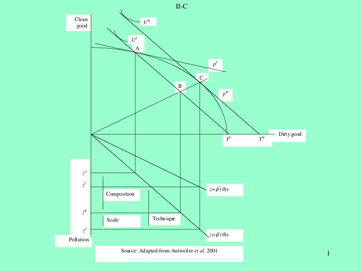
II-C Externalities • E.g. env. externality in production • TEF is now: • e(p, u) = r(p, v) - z'y • where z is qty of pollution per unit of y produced. • Env. externality in consumption: • u = u(c, z) ==> e(p, z, u) • NB assumption of separability.
II-C Non-traded goods • Goods may be non-traded (or effectively so) for intrinsic and policy reasons. • If one good is non-traded, for this, mn = 0. Equilibrium now requires additional equation: e(p, u) = r(p, v) en(p, u) = rn(p, v) and solves for pn as well as agg. welfare. • With endogenous prices, preferences play a role in economic structure.
II-C Salter-Swann diagram T RER = pN/pT (yT, yN) = (cT, cN) N
II-C Effects of growth with non-traded good T Income exp. path N
II-C Two fundamental GE results • Distributional effects of a price change: the Stolper-Samuelson theorem • Production effects of a factor endowment change: the Rybczinski theorem • Assume: • Two factors of production, two products, so yj = yj(x1, x2), for j = 1,2 • Complete and competitive markets, CRTS. • Prices are ‘given’ in world markets.
II-C A useful tool: ‘hat’ calculus
II-C Effects of a price change
II-C Stolper-Samuelson theorem A rise in one commodity price raises the real return to the factor used intensively in producing that commodity, and reduces the real return to the other factor.
II-C Applications of S-S • Effects of trade shocks or trade policy reforms on the returns to factors • For environmental analysis: changes in factor returns indicate incentives for exploitation or investment • Ex.1: If forests are open-access, a ‘shock’ that raises returns to timber may increase harvests • Ex. 2: raising returns to agriculture may promote soil-conserving investments
II-C Effects of endowment growth
II-C Rybczinski Theorem At constant prices, expansion of one factor endowment raises output of the good that uses that factor intensively, and reduces that of the other good. If 2 factors expand, one good's output grows more slowly than the rate of growth of either factor.
II-C Implications of Ryb. result • Unequal rates of factor accumulation alter structure of production • Capital deepening causes labor-intensive or NR-intensive sectors to decline, other things equal • Thus investment in non-agricultural sectors may diminish pressures exerted on the natural resource base by primary industries.
II-C Discussion of fundamental results • The S-S and R theorems provide ‘core’ insights for any GE analysis. • They hold for 2X2 models; similar, but weaker predictions apply for higher-dimension models. • Both theorems break down in presence of externalities. • In practice, however, can use these predictions to check the credibility of predictions obtained from larger models.