Download
1 / 31
340 likes | 551 Views
Basic Statistical Concepts. Psych 231: Research Methods in Psychology. Turn in Journal summary #2 in class on Wednesday (moved from turning in last week in labs). There are three main measures of center Mean (M) : the arithmetic average Add up all of the scores and divide by the total number

E N D
Basic Statistical Concepts Psych 231: Research Methods in Psychology
Turn in Journal summary #2 in class on Wednesday (moved from turning in last week in labs)
There are three main measures of center • Mean (M): the arithmetic average • Add up all of the scores and divide by the total number • Most used measure of center • Median (Mdn): the middle score in terms of location • The score that cuts off the top 50% of the from the bottom 50% • Good for skewed distributions (e.g. net worth) • Mode: the most frequent score • Good for nominal scales (e.g. eye color) • A must for multi-modal distributions Properties of distributions: Center
Divide by the total number in the population Add up all of the X’s Divide by the total number in the sample • The most commonly used measure of center • The arithmetic average • Computing the mean • The formula for the population mean is (a parameter): • The formula for the sample mean is (a statistic): The Mean
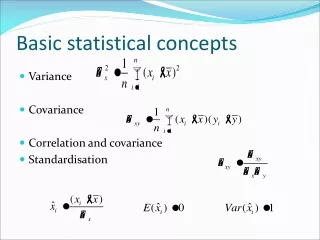
How similar are the scores? • Range: the maximum value - minimum value • Only takes two scores from the distribution into account • Influenced by extreme values (outliers) • Standard deviation (SD): (essentially) the average amount that the scores in the distribution deviate from the mean • Takes all of the scores into account • Also influenced by extreme values (but not as much as the range) • Variance: standard deviation squared Spread (Variability)
mean mean Low variability The scores are fairly similar High variability The scores are fairly dissimilar 50, 51, 48, 54, 52, 47, 45 30, 51, 38, 64, 52, 47, 65 Variability
m • The standard deviation is the most popular and most important measure of variability. • The standard deviation measures how far off all of the individuals in the distribution are from a standard, where that standard is the mean of the distribution. • Essentially, the average of the deviations. Standard deviation
1 2 3 4 5 6 7 8 9 10 m Our population 2, 4, 6, 8 An Example: Computing the Mean
-3 1 2 3 4 5 6 7 8 9 10 m • Step 1: To get a measure of the deviation we need to subtract the population mean from every individual in our distribution. Our population 2, 4, 6, 8 X - = deviation scores 2 - 5 = -3 An Example: Computing Standard Deviation (population)
-1 1 2 3 4 5 6 7 8 9 10 m • Step 1: To get a measure of the deviation we need to subtract the population mean from every individual in our distribution. Our population 2, 4, 6, 8 X - = deviation scores 2 - 5 = -3 4 - 5 = -1 An Example: Computing Standard Deviation (population)
1 1 2 3 4 5 6 7 8 9 10 m • Step 1: To get a measure of the deviation we need to subtract the population mean from every individual in our distribution. Our population 2, 4, 6, 8 X - = deviation scores 2 - 5 = -3 6 - 5 = +1 4 - 5 = -1 An Example: Computing Standard Deviation (population)
3 1 2 3 4 5 6 7 8 9 10 m • Step 1: To get a measure of the deviation we need to subtract the population mean from every individual in our distribution. Our population 2, 4, 6, 8 X - = deviation scores 2 - 5 = -3 6 - 5 = +1 Notice that if you add up all of the deviations they must equal 0. 4 - 5 = -1 8 - 5 = +3 An Example: Computing Standard Deviation (population)
X - = deviation scores 2 - 5 = -3 6 - 5 = +1 4 - 5 = -1 8 - 5 = +3 • Step 2: So what we have to do is get rid of the negative signs. We do this by squaring the deviations and then taking the square root of the sum of the squared deviations (SS). SS = (X - )2 + (+3)2 = (-3)2 + (-1)2 + (+1)2 = 9 + 1 + 1 + 9 = 20 An Example: Computing Standard Deviation (population)
Step 3: ComputeVariance (which is simply the average of the squared deviations (SS)) • So to get the mean, we need to divide by the number of individuals in the population. variance = 2 = SS/N = 20/4 = 5.0 An Example: Computing Standard Deviation (population)
standard deviation = = • Step 4: Compute Standard Deviation • To get this we need to take the square root of the population variance. An Example: Computing Standard Deviation (population)
To review: • Step 1: Compute deviation scores • Step 2: Compute the SS • Step 3: Determine the variance • Take the average of the squared deviations • Divide the SS by the N • Step 4: Determine the standard deviation • Take the square root of the variance An Example: Computing Standard Deviation (population)
To review: • Step 1: Compute deviation scores • Step 2: Compute the SS • Step 3: Determine the variance • Take the average of the squared deviations • Divide the SS by the N-1 • Step 4: Determine the standard deviation • Take the square root of the variance • This is done because samples are biased to be less variable than the population. This “correction factor” will increase the sample’s SD (making it a better estimate of the population’s SD) An Example: Computing Standard Deviation (sample)
Example: Suppose that you notice that the more you study for an exam, the better your score typically is. • This suggests that there is a relationship between study time and test performance. • We call this relationship a correlation. Relationships between variables
Properties of a correlation • Form (linear or non-linear) • Direction (positive or negative) • Strength (none, weak, strong, perfect) • To examine this relationship you should: • Make a scatterplot • Compute the Correlation Coefficient Relationships between variables
Plots one variable against the other • Useful for “seeing” the relationship • Form, Direction, and Strength • Each point corresponds to a different individual • Imagine a line through the data points Scatterplot
Y 6 5 4 3 2 1 1 2 3 4 5 6 X Scatterplot
A numerical description of the relationship between two variables • For relationship between two continuous variables we use Pearson’s r • It basically tells us how much our two variables vary together • As X goes up, what does Y typically do • X, Y • X, Y • X, Y Correlation Coefficient
Linear Non-linear Form
Y Y X X Positive Negative • As X goes up, Y goes up • X & Y vary in the same direction • Positive Pearson’s r • As X goes up, Y goes down • X & Y vary in opposite directions • Negative Pearson’s r Direction
Zero means “no relationship”. • The farther the r is from zero, the stronger the relationship • The strength of the relationship • Spread around the line (note the axis scales) Strength
r = 1.0 “perfect positive corr.” r = 0.0 “no relationship” -1.0 0.0 +1.0 The farther from zero, the stronger the relationship r = -1.0 “perfect negative corr.” Strength
r = -0.8 r = 0.5 -.8 .5 -1.0 0.0 +1.0 Rel A Rel B • Which relationship is stronger? • Rel A, -0.8 is stronger than +0.5 Strength
Y 6 5 4 3 2 1 1 2 3 4 5 6 X 0.5 2.0 Change in Y Change in X = slope • Compute the equation for the line that best fits the data points Y = (X)(slope) + (intercept) Regression
Y 6 5 4 3 2 4.5 1 1 2 3 4 5 6 X • Can make specific predictions about Y based on X X = 5 Y = ? Y = (X)(.5) + (2.0) Y = (5)(.5) + (2.0) Y = 2.5 + 2 = 4.5 Regression
Y Y 6 6 5 5 4 4 3 3 2 2 1 1 1 1 2 2 3 3 4 4 5 5 6 6 X X • Also need a measure of error Y = X(.5) + (2.0) + error Y = X(.5) + (2.0) + error • Same line, but different relationships (strength difference) Regression
Don’t make causal claims • Don’t extrapolate • Extreme scores (outliers) can strongly influence the calculated relationship Cautions with correlation & regression