Download
1 / 34
340 likes | 377 Views
Basic statistical concepts. Variance Covariance Correlation and covariance Standardisation. Factor Analysis & Principal Component Analysis.

E N D
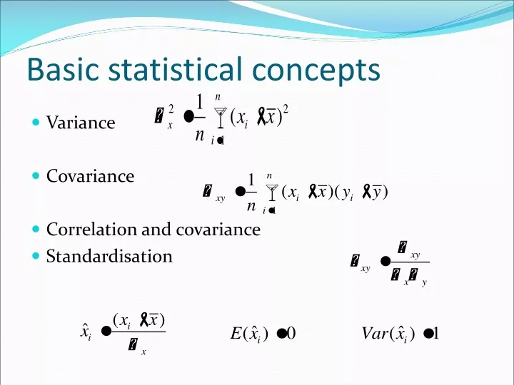
Basic statistical concepts • Variance • Covariance • Correlation and covariance • Standardisation
Factor Analysis & Principal Component Analysis A statistical procedure for “data reduction”, i.e. summarising a given set of variables into a reduced set of unrelated variables, explaining most of the original variability Objectives • Identification of a smaller set of unrelated variables replacing the original set • Identification of underlying factors explaining correlation among variables • Selection of a smaller set of proxy variables
Key concepts for factor analysis • What is summarised is the variability of the original data set • There is no observed dependent variable as in regression, but interdependence (correlation) is explored • Each variable is explained by a set of underlying (non observed/latents) factors • Each underlying factor (latent variable) is explained by the original set of variables • Hence... Each variable is related to the remaining variables (interdependence)
Factor Analysis & PCA • In principal components analysis,the total variance in the data is considered. Principal components analysis is recommended when the primary concern is to determine the minimum number of factors that will account for maximum variance in the data for use in subsequent multivariate analysis. The factors are called principal components. • STATA COMMAND: pca • Infactor analysis,the factors are estimated based only on the common variance. This method is appropriate when the primary concern is to identify the underlying dimensions and the common variance is of interest. • STATA COMMAND: factor
Factor analysis Total Common Unique Error variability variability variability variability µ X = +f(F ) +e j j k j µ Var(X)=Var( )+Var(F)+Var(e) Correlation Matrix for {X } j
Factor analysis model X1 = m1 + g11F1+ g12F2+… + g1mFm+e1 X2 = m2 + g21F1+ g22F2+… + g2mFm+e2 Xj = mj + gj1F1+ gj2F2+… + gjmFm+ej Xp = mp + gp1F1+ gp2F2+… + gpmFm+ep X = m + GF + e where Fi (i=1,2,…,m) are uncorrelated random variables (common variability/ factors) mp mi (i=1,2,…,p) are unique factors for each variable – Unique variability ei (i=1,2,…,p) are error random variables, uncorrelated with each other and with F and represent the residual error due to the use of common factors – Error variability
Factor analysis model (factors view) F1 = b11X1+ b12X2+… + b1pXp F2 = b21X1+ b22X2+… + b2pXp Fj = bj1X1+ bj2X2+… + bjpXp Fm = bp1X1+ bp2X2+… + bppXp F = bX The common factors are linear combinations of the original variables
Estimation • There is not an unique solution (set of common factors) – any “orthogonal rotation” of the solution is acceptable (factor rotation) • Variables in X need to be standardised prior to analysis • Factor analysis estimate the following quantities: • The simple correlations (covariance) between each factor i and the original variables j (factor loadings), i.e. the coefficients gij (the factor or component matrix) • The values of each common factor, for each of the statistical units (factor scores)
Problem formulation Construction of the Correlation Matrix Method of Factor Analysis Determination of Number of Factors Rotation of Factors Interpretation of Factors Selection of Surrogate Variables Calculation of Factor Scores Determination of Model Fit Conducting Factor Analysis
Some terminology • Communality. Communality is the amount of variance a variable shares with all the other variables being considered. This is also the proportion of variance explained by the common factors. • Eigenvalue. The eigenvalue represents the total variance explained by each factor. • Factor loadings. Factor loadings are simple correlations between the variables and the factors.
Construct/check the Correlation Matrix • The analytical process is based on a matrix of correlations between the variables. • Bartlett's test of sphericity can be used to test the null hypothesis that the variables are uncorrelated in the population: in other words, the population correlation matrix is an identity matrix. If this hypothesis cannot be rejected, then the appropriateness of factor analysis should be questioned. • STATA command: factortest
Checking correlation matrix: Bartlett’s test STATA command: factortest Since significance level for Bartlett’s test < 0.05, reject null hypothesis → appropriate to apply factor analysis to these data
Initial Run • A preliminary run that includes a full set of factors is necessary so that a smaller set can be chosen based on certain criteria. • In intial run, principal components will extract as many factors as there are variables
Determine the Number of Factors • A Priori Determination. Sometimes, because of prior knowledge, the researcher knows how many factors to expect and thus can specify the number of factors to be extracted beforehand. • Determination Based on Eigenvalues. In this approach, only factors with Eigenvalues greater than 1.0 are retained. An Eigenvalue represents the amount of variance associated with the factor. Hence, only factors with a variance greater than 1.0 are included. Factors with variance less than 1.0 are no better than a single variable, since, due to standardization, each variable has a variance of 1.0.
Determine the Number of Factors • Determination Based on Scree Plot.A scree plot is a plot of the Eigenvalues against the number of factors in order of extraction. Experimental evidence indicates that the point at which the scree begins denotes the true number of factors. • Determination Based on Percentage of Variance.In this approach the number of factors extracted is determined so that the cumulative percentage of variance extracted by the factors reaches a satisfactory level. It is recommended that the factors extracted should account for at least 60% of the variance.
Rotate Factors • Although the initial or unrotated factor matrix indicates the relationship between the factors and individual variables, it seldom results in factors that can be interpreted, because the factors are correlated with many variables. Therefore, through rotation the factor matrix is transformed into a simpler one that is easier to interpret. • In rotating the factors, we would like each factor to have nonzero, or significant, loadings or coefficients for only some of the variables. Likewise, we would like each variable to have nonzero or significant loadings with only a few factors, if possible with only one.
Rotate Factors • The most commonly used method for rotation is the varimax procedure. This is an orthogonal method of rotation that minimizes the number of variables with high loadings on a factor, thereby enhancing the interpretability of the factors. (Orthogonal rotation results in factors that are uncorrelated) STATA COMMAND (after pca, factor) rotate, varimax blank(0.4)
Factors Factors Variables 1 2 3 4 5 6 1 X X X 2 X X X Variables 1 2 3 4 5 6 1 X X X X X 2 X X X X (a) (b) High Loadings Before Rotation High Loadings After Rotation Factor Matrix Before and After Rotation: Example
Factor scores & surrogate variables • For each household/person in sample, STATA will calculate a value for each factor: the factor scores. These can be used in further analysis • By examining the factor matrix, one could select for each factor the variable with the highest loading on that factor. That variable could then be used as a surrogate/proxy variable for the associated factor in further analysis • STATA COMMAND (after pca or factor) : predict
Cluster Analysis • It is a class of techniques used to classify cases into groups that are relatively homogeneous within themselves and heterogeneous between each other, on the basis of a defined set of variables. These groups are called clusters. • Usually used to group subjects/objects/cases (eg. Shoppers, households, geographical regions, products, brands, etc.), unlike factor analysis, which combines variables.
Cluster Analysis and marketing research • Market segmentation. E.g. clustering of consumers according to their attribute preferences • Understanding buyer behaviours. Consumers with similar behaviours/characteristics are clustered • Identifying new product opportunities. Clusters of similar brands/products can help identify competitors / market opportunities • Geographical segmentation: Clustering of cities or regions or supermarket outlets on the basis of various characteristics and outcomes. • Reducing data. E.g. in preference mapping
Defining Distance • Most common: Euclidean. Dij distance between cases i and j xkivalue of variable Xkfor case j The Euclidean distance is the square root of the sum of the squared differences in values for each variable. • Others include the city-block or Manhattan: distancebetween two objects is the sum of the absolute differences in values for each variable. • Should also standardize all variables in analysis to have mean 0 and variance 1 to prevent misleading results.
Clustering Procedures Hierarchical Nonhierarchical Other Agglomerative Divisive Two-Step Centroid Sequential Parallel Optimizing Linkage Variance Methods Threshold Threshold Partitioning Methods Methods Ward’s Method Single Complete Average Linkage Linkage Linkage Choosing a clustering procedure
3. Clustering procedures • Hierarchical procedures • Agglomerative (start from n clusters, to get to 1 cluster) • Divisive (start from 1 cluster, to get to n clusters) • Non hierarchical procedures • K-means clustering
3. Agglomerative clustering • Linkage methods • Single linkage (minimum distance) • Complete linkage (maximum distance) • Average linkage • Ward’s method • Compute sum of squared distances within clusters • Aggregate clusters with the minimum increase in the overall sum of squares • Centroid method • The distance between two clusters is defined as the difference between the centroids (cluster averages)
Single Linkage Minimum Distance Cluster 2 Cluster 1 Complete Linkage Maximum Distance Cluster 1 Cluster 2 Average Linkage Average Distance Cluster 1 Cluster 2 3. Linkage Methods of Clustering
Ward’s Procedure Centroid Method 3. Other Agglomerative Clustering Methods
Non-hierarchical: K-means clustering • The number k of clusters is fixed • An initial set of k “seeds” (aggregation centres) is provided • Given a certain threshold, all units are assigned to the nearest cluster seed • New seeds are computed • Go back to step 3 until no reclassification is necessary Units can be reassigned in successive steps (optimising partioning)
3. Hierarchical vs Non hierarchical methods Hierarchical clustering • No decision about the number of clusters • Problems when data contain a high level of error • Can be very slow • Initial decisions are more influential (one-step only) • Non hierarchical clustering • Faster, more reliable • Need to specify the number of clusters (arbitrary)
A Suggested approach – Two step • First perform a hierarchical method to define the number of clusters • Then use the k-means procedure to actually form the clusters
Cluster analysis: basic steps • Apply Ward’s methods • STATA COMMAND cluster wards var1 var2 var3 varn , name(nameclust) cluster dendrogram nameclust, labels(var) xlabel(, angle(90) ) • Check the agglomeration schedule • Decide the number of clusters • Apply the k-means method cluster kmeans var1 var2 var3 varn , k(numcluster)
Interpret & Profile • For each cluster, look at cluster average values for each variable. Compare to other clusters and interpret accordingly. • ‘cluster membership’ variable can be used to relate to other variables in further step.