Elasticity of Demand and Supply

1. Elasticity of Demand and Supply ECO 2023 Chapter 6 Fall 2007

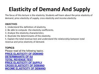
2. Price Elasticity of Demand • Law of demand tells us that consumers will buy more of a product when its price declines and less when its price increases. • How much? Varies from product to product and over different price ranges for the same product. • The responsiveness of consumers to a change in the price of a product is measured by the Price Elasticity of Demand. • Some products are more responsive than others.

3. Price Elasticity of Demand • Percentage change in quantity demanded divided by the percentage change in price • Ed = % change in quantity demanded % change in price

4. Mathematical Example • Suppose that Price goes from $1.10 to $0.90, causing quantity demanded to change from 95,000 to 105,000 • Ed = (10,000/(95,000 + 105,000)/2 ÷ ($1.00/($1.10 + $0.90)/2 = 10%/-20% = -50%

5. Interpretations • Elastic Demand • Change in Price < Change in Quantity Demanded • E > 1 • The change in price is less than the change in the quantity demanded. • TVs • If price decreases then total revenue increases. • Luxuries • Many substitutes • Price and total revenue moves in opposite directions

6. Elastic Demand Price $5 $4 Demand Quantity 200 300

7. Perfectly Elastic Demand • Change in Price: causes a infinite change in quantity demanded • E =  • Horizontal demand curve exists • A small reduction in price will cause buyers to purchase from ZERO to all they can • If price changes then there is no quantity demanded by consumers • Wheat

8. Perfectly Elastic Demand Price $4 Demand Quantity 200 300

9. Inelastic Demand • Change in Price > Change in Quantity Demanded • E < 1 • The change in price is greater than the change in the quantity demanded. • Electricity • Necessities

10. Inelastic Demand Price • Relatively inelastic demand • A somewhat vertical line • Any price change has little effect on the quantity demanded • Ed < 0 • Few substitutes • Electricity P1 P2 Demand Q1 Q2 Q

11. Inelastic Demand Price • Perfectly Inelastic Demand • A vertical line • Any price change has no effect on the quantity demanded • Ed = 0 • No substitutes • Insulin P1 P2 Demand Q

12. Unit Elasticity P • Everywhere along the demand curve • percentage change in price = percentage change in Quantity demanded • No change in total revenue • E = 1 • Movies Demand Q

13. Total Revenue • The importance of elasticity for firms relates to the effect of price changes on total revenue and thus on profits. • Profits = Total revenue – Total cost • Total revenue = Price X Quantity • Total revenue and price elasticity of demand are related. The relationship will tell you if demand is elastic or inelastic.

14. Total Revenue & Elastic Demand • If demand is elastic, a decrease in price will increase total revenue • Even though a lesser price is received per unit, enough additional units are sold to more than make up for the lower price. • For example: • Price of TVs is $200 per unit and 600 units is sold. • Now price of the TVs is $150 per unit and 900 units are sold • Total revenue = P X Q = $200 X 600 = $120,000 • Total revenue = $150 X 900 = $135,000 • Revenue increased by $15,000

15. Total Revenue & Inelastic Demand • If demand is inelastic, a price decrease will reduce total revenue. • The modest increase in price will not offset the decline in revenue per unit. • For example: • Price of insulin is $9 per injection and 1,000 units are sold • Price of insulin decreases to $7 per injection and 1,100 units are sold • Total revenue = $9 X 1,000 = $9,000 • Total revenue = $7 X 1,100 = $7,700 • Total revenue decreases $1,300

16. Total Revenue & Unitary Elastic • An increase or decrease in the price leaves total revenue unchanged. • The loss in revenue from a lower price is exactly offset by the gain in revenue from accompanying increase in sales. • For example: • Price of movie tickets is $6 per ticket and 1,000 tickets are sold • Price of movie tickets goes to $5 per ticket and 1,200 tickets are sold • Total revenue = $6 X 1,000 = $6,000 • Total revenue = $5 X 1,200 = $6,000 • No change in total revenue

17. Determinants of Elasticity of Demand • Substitutability • The larger the number of substitute goods that are available, the greater the price elasticity of demand • Proportion of income • The higher the price of a good relative to consumers’ income, the greater the price elasticity of demand • Luxuries vs. necessities • The more that a good is considered to be a luxury rather than a necessity the greater is the price elasticity of demand • Time • Product demand is more elastic the longer the time period under consideration

18. Price Elasticity of Supply • Law of supply tells us that producers will respond to a decline in prices with a decrease in quantity supplied. • The responsiveness of suppliers to a change in the price of a product is measured by the Price Elasticity of Supply. • Some products are more responsive than others. • If producers are relatively responsive to price changes, supply is elastic • If they are relatively insensitive to price changes, supply is inelastic

19. Price Elasticity of Supply • Ed = % change in quantity supplied % change in price

20. Price Elasticity of Supply • The Market Period: • Is the period that occurs when the time immediately after a change in market price is too short for producers to respond with a change in quantity supplied. • Therefore, elasticity of supply is perfectly inelastic during this period • Short run: • The plant capacity of individual producers and of the entire industry is fixed. • Firms do have to use their fixed plants more or less intensively • Elastic supply • Long Run: • Is a time period long enough for firms to adjust their plant sizes and for new firms to enter or existing firms to leave the industry • More elastic supply

21. Cross Elasticity of Demand • Measures how sensitive consumer purchases of one product are to a change in the price of some other product • Substitutes: if cross elasticity of demand is POSITIVE, meaning that sales of X move in the same direction as a change in the price of Y then X ad Y are substitutes • Complementary goods: when cross elasticity is NEGATIVE. We know that X and Y go together, an increase in the price of one decreases the demand for the other • Independent goods: a zero or near zero cross elasticity suggests that the two products being considered as unrelated or independent goods.

22. Income Elasticity of Demand • Measures the degree to which consumers respond to a change in their incomes by buying more or les of a particular good. • Normal goods – Ei > 1 • meaning that more of the good is demanded as incomes rise • Inferior goods - Ei < 1 • Meaning that less of the good is demanded as incomes rises

23. Consumer Surplus • The benefit surplus received by a consumer or consumers in a market. • It is the difference between the maximum price a consumer is willing to pay for a product and the actual price. • The utility surplus = consumers receive a greater total utility in dollar terms from their purchases than the amount of their expenditures from their purchases than the amount of their expenditures • This is caused because all consumers pay the equilibrium price even though many would be willing to pay more than that price to obtain the product.

24. Consumer Surplus Equilibrium Eq. Price Demand Eq. Quantity Consumer Surplus

25. Consumer Surplus • Example: Suppose that a product sells for an equilibrium price of $8. Here are consumers willingness to pay.

26. Consumer Surplus • Consumer surplus and price are inversely related. Higher prices reduce consumer surplus, lower prices increase it.

27. Producer Surplus • Is the difference between the actual price a producer receives and the minimum acceptable price. • Sellers collectively receive a producer surplus in most markets because most sellers are willing to accept a lower than equilibrium price if that is required in order to sell the product.

28. Equilibrium Price Supply Producer Surplus Producer Surplus

29. Producer’s Surplus • There is a direct relationship between equilibrium price and the amount of producer surplus. • Lower prices reduce producer surplus and higher prices increase it.

30. Equilibrium Price Supply Demand Consumer surplus Producer’ Surplus Efficiency

31. Efficiency • All markets that have downward sloping demand curves and upward sloping supply curves yield consumer and producer surplus. • Equilibrium quantity reflects economic efficiency. • Productive efficiency is achieved because competition forces producers to use the best techniques and combinations of resources. Production costs are minimized

32. Efficiency • Allocative Efficiency is achieved because the correct quantity of output is produced relative to other goods and services. • Occurs when • Marginal benefit = Marginal cost • Maximum willingness to pay = minimum acceptable price • Combined consumer and producer surplus is at a maximum.

33. Efficiency Losses • Reductions in combined consumer and producer surplus associated with underproduction or overproduction of a product. • Called deadweight losses