Download
1 / 16
200 likes | 660 Views
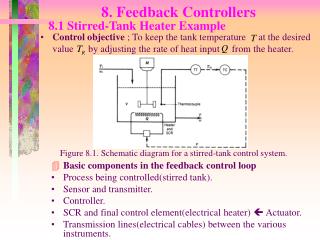
Control objective ; To keep the tank temperature at the desired value by adjusting the rate of heat input from the heater. 8. Feedback Controllers. 8.1 Stirred-Tank Heater Example. Basic components in the feedback control loop Process being controlled(stirred tank).

E N D
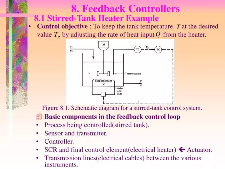
Control objective ; To keep the tank temperature at the desired value by adjusting the rate of heat input from the heater. 8. Feedback Controllers 8.1 Stirred-Tank Heater Example • Basic components in the feedback control loop • Process being controlled(stirred tank). • Sensor and transmitter. • Controller. • SCR and final control element(electrical heater) Actuator. • Transmission lines(electrical cables) between the various instruments. Figure 8.1. Schematic diagram for a stirred-tank control system.
Transmission line Controller Actuator Process Sensor 8.2 Controller Implementation Using PC Figure 8.2. Typical equipment for process control using computer.
8.3 Controllers 8.3.1 Historical Perspectives 250 B.C ; Greeks, water level controller Their mode of operation was very similar to that of the level regulator in the modern flush toilet. 1788 ; James Watt, fly-ball governor It played a key role in the development of stream power. 1930s ; PID controller became commercially available The first theoretical papers on process control were published. 1940s ; Pneumatic PID controller 1950s ; Electronic PID controller Late 1950 ~ 1960s ; The first computer control applications
8.3.2 PID Controllers • PID controller is the controller that has the three basic control modes of Proportional(P), Integral(I) , and Derivative(D). • PID controllers are still used widely in industry because of their simplicity, robustness, and successful practical applications. • In spite of the development of many advanced control algorithms, nearly 80% of the controllers in the industrial field are PID controller. Figure 8.3. Flow control system. Figure 8.4. Schematic diagram of a feedback controller.
Proportional(P) part: Integral(I) part: Derivative(D) part: Where and denote the set point(the desired process output) and process out put. Constants are called proportional gain, integral time and derivative time, respectively. 8.3.2.1 Structure of PID Controllers. • Three parts of the PID controller : • PID controller is sum of the above three part as follows.
8.3.2.2 Roles of Three Parts • Proportional part : Since the control output( ) is proportional to the error , it plays role in pushing the process output to the set point as much as the error. 1. Transfer function. 2. Advantage : immediate corrective action. 3. Disadvantage : steady-state error(offset). 4. Usage : when the steady-state error is tolerable( ex. level control which wants to prevent the system from overflowing or drying), proportional-only controller is attractive because of its simplicity seldom used only. To remove the steady-state error(offset), the integral control action should be included in the feedback controller.
Steady-state error. For usual process(i.e., open-loop stable processes), the control output should be nonzero to keep the process output in a nonzero set point. • Consider the following PD controller( the following derivation is applicable to P controller case). PD(or P) controller output is always zero at steady-state if the error is zero(i.e., ). • PD(or P) controller cannot be nonzero constant when the error is zero at steady-state. So, the PD(or P) controller cannot keep the process output in a nonzero set point for open-loop stable processes. • Offset can be calculated as follows. Here denotes steady state and is the static gain(or DC gain) of the process.
1. Transfer function. • Integral part(= reset or floating control part) : Since the integral part is not necessarily zero even though the error at steady-state is zero, it plays an important role in rejecting the offset. 2. Disadvantages Not immediate corrective action. Practically PI controller is used. Oscillatory response. Reduce the stability of the system. Solution ; proper tuning of the controller or including derivative control action which tends to counteract the destabilizing effects. Reset windup( or integral windup).
Reset windup( or Integral windup). • Sustained error Large integral term Saturation of controller output Further buildup of the integral term while the controller is saturated is referred to as reset windup or integral windup. • Reset windup occurs when a PI or PID controller encounters a sustained error, for example, during the start-up of a batch process or after a large set-point change. • The large overshoot occurs because the integral term continues to increase until the error signal changes sign at . • Antireset windup ; halting the integral action whenever the controller output saturates. Most of commercial controllers provides antireset windup. Figure 8.5. Reset windup during a set-point change.
1. Transfer function. 2. Advantage : This part enhance the robustness of the PID controller by considering abrupt change of the error. Figure 8.6. Extrapolation using the derivative of the error • Derivative part(= rate action,pre-act or anticipatory control part) : Since this part represents approximately the increment of the error after time from the present time , it plays a role in rejecting the future error in advance by increasing the control output proportional to the future incremental error. 3. Disadvantage : If the process measurement is noisy, this term will change widely and amplify the noise unless the measurement is filtered.
Electronic or pneumatic device that provides ideal derivative action cannot be built(is physically unrealizable). Commercial controllers approximate the ideal behavior as follows. where is a small number, typically between 0.05 and 0.2. 8.3.2.3 Ideal PID Controller. 1. Transfer function. 2. Disadvantages. Derivative kick Proportional kick
8.3.3 On-Off Controllers • The controller output of ideal on-off controller. where and denote the on and off values, respectively. • On-off controller can be considered to be a special case of P controller with a very high controller gain • Advantage : Simple and inexpensive controllers. • Disadvantage Not versatile and ineffective. Continuous cycling of the controlled variable and excess wear on the final control element. • Usage : Thermostats in heating system. Domestic refrigerator. Noncritical industrial applications.
8.3.4 Typical Response of Feedback Control Systems • No feedback control make the process slowly reach a new steady-state. • Proportional control speeds up the process response and reduces the offset. • Integral control eliminates offset but tends to make the response oscillatory. • Derivative control reduces both the degree of oscillation and response time. Figure 8.7. Typical process response with feedback control. C is the deviation from the initial steady-state.
8.3.4.1 Effect of controller gain . • Increasing the controller gain. less sluggish process response. • Too large controller gain. undesirable degree of oscillation or even unstable response. • An intermediate value of the controller gain best control result. Figure 8.8. Process response with proportional control.
8.3.4.2 Effect of integral time . • Increasing the integral time. more conservative(sluggish) process response. • Too large integral time. too long time to reach to the set point after load upset or set-point change occurs. • Theoretically, offset will be eliminated for all values of . Figure 8.9. PI control: (a) effect of integral time (b) effect of controller gain.
8.3.4.3 Effect of derivative time . Figure 8.10. PID control: effect of derivative time. • Increasing the derivative time. improved response by reducing the maximum deviation, response time and the degree of oscillation. • Too large derivative time. measurement noise tends to be amplified and the response may be oscillatory. • Intermediate value of is desirable.