Download
1 / 24
250 likes | 509 Views
OLS Regression. What is it? Closely allied with correlation – interested in the strength of the linear relationship between two variables One variable is specified as the dependent variable The other variable is the independent (or explanatory) variable. Regression Model Y = a + bx + e

E N D
OLS Regression • What is it? • Closely allied with correlation – interested in the strength of the linear relationship between two variables • One variable is specified as the dependent variable • The other variable is the independent (or explanatory) variable
Regression Model • Y = a + bx + e • What is Y? • What is a? • What is b? • What is x? • What is e? • What is Y-hat?
Elements of the Regression Line • a = Y intercept (what Y is predicted to equal when X = 0) • b = Slope (indicates the change in Y associated with a unit increase in X) • e = error (the difference between the predicted Y (Y hat) and the observed Y
Regression • Has the ability to quantify precisely the relative importance of a variable • Has the ability to quantify how much variance is explained by a variable(s) • Use more often than any other statistical technique
The Regression Line • Y = a + bx + e • Y = sentence length • X = prior convictions • Each point represents the number of priors (X) and sentence length (Y) of a particular defendant • The regression line is the best fit line through the overall scatter of points
Calculus 101 Least Squares Method and differential calculus Differentiation is a very powerful tool that is used extensively in model estimation. Practical examples of differentiation are usually in the form of minimization/optimization problems or rate of change problems.
Calculus 101: Calculating the rate of change or slope of a line For a straight line it is relatively simple to calculate the slope
Calculating the rate of change or slope of a line for a curve is a bit harder Differential Calculus: We have a curve describing the variable Y as some function of the variable X: y = x2
It is possible to find a general expression involving the function f(x) that describes the slopes of the approximating sequence of secant lines h = x1 – x0 (represents a small difference from a point of interest)
Lets take a cost curve example: C(x) = x2 what is the derivative if x = 3 = f(3+h) – f(3) / h = (3+h)2 – (3)2 / h = (9 + 6h + h2) – 9 / h = 6h + h2 / h = 6 + h = 6 (as h approaches 0) ∆y/∆x = 6
How does this relate to our Regression model that is a straight line?
How do you draw a line when the line can be drawn in almost any direction? The Method of Least Squares: drawing a line that minimizing the squared distances from the line (Σe2) This is a minimization problem and therefore we can use differential calculus to estimate this line.
Summing the squares of the deviations yields: • f(a, b) = 55-30a + 5a2 - 78b + 20ab + 30b2 • Calculate the first order partial derivatives of f(a,b) • fb = -78 + 20a + 60b and fa = -30 + 10a + 20b
Set each partial derivative to zero: Manipulate fa: • 0 = -30 + 10a + 20b • 10a = 30 - 20b • a= 3 - 2b
Substitute (3-2b) into fb: • 0 = -78 + 20a + 60b = -78 +20(3-2b) + 60b • = -78 + 60 - 40b + 60b • = -18 +20b • 20b = 18 • b = 0.9 • Slope = .09
Substituting this value of b back into fa to obtain a: • 10a = 30 - 20(.09) • 10a = 30 - 18 • 10a = 12 • a= 1.2 • Y-intercept = 1.2
Estimating the model (the easy way) Calculating the slope (b)
Sum of Squares for X • Some of Squares for Y • Sum of produces
Calculating the Y-intersept (a) Calculating the error term (e) Y hat = predicted value of Y e will be different for every observation. It is a measure of how much we are off in are prediction.