Download
1 / 12
120 likes | 248 Views
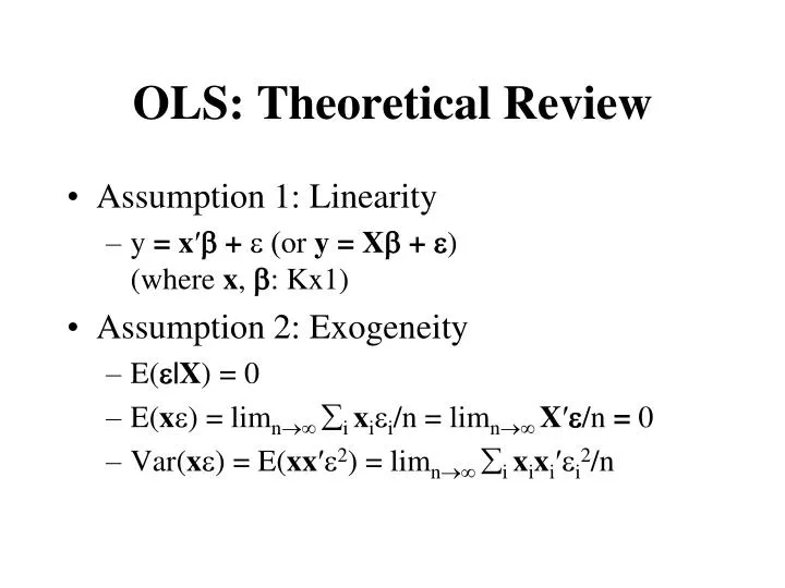
OLS: Theoretical Review. Assumption 1: Linearity y = x ′ b + e ( or y = X b + e ) (where x , b : Kx1) Assumption 2: Exogeneity E( |X ) = 0 E( x ) = lim n i x i e i /n = lim n X ′ /n = 0 Var( x ) = E( xx ′ 2 ) = lim n i x i x i ′ e i 2 /n.

E N D
OLS: Theoretical Review • Assumption 1: Linearity • y = x′b + e(or y = Xb + e) (where x, b: Kx1) • Assumption 2: Exogeneity • E(|X) = 0 • E(x) = limn i xiei/n = limn X′/n = 0 • Var(x) = E(xx′2) = limn i xixi′ei2/n
OLS: Theoretical Review • Assumption 3: No Multicolinearity • rank(X) = K • E(xx') = limnixixi′/n = limnX′X/n • plim X’X/n exists and nonsingular
OLS: Theoretical Review • Non-Spherical Disturbances: General Heteroschedasticity • Var(e) = • Var(xe) = E(xx′e2) = limnX′X/n • X′e/n dN(0,X′X/n)
OLS: Theoretical Review • Assumption 4: Homoschedasticity andNo Autocorrelation • Var(e) = s2I • Var(xe) = E(xx′e2) = limns2X′X/n • X′e/n dN(0, s2X′X/n)
OLS: Theoretical Review • Least Squares Estimator • b = (X'X)-1X'y • Variance-Covariance Matrix of b • General Heteroscedasticity:Var(b) = (X'X)-1X′X(X'X)-1 • Homoschedasticity: Var(b) = 2(X'X)-1
OLS: Theoretical Review • Least Squares Estimator • b = (X'X/n)-1(X'y/n) • b = + (X'X/n)-1(X'/n), bp • n(b - ) = (X'X/n)-1(X'/n) • n(b - ) dN(0,A-1BA-1)A = E(xx′) = limnX'X/nB = E(xx′e2) = limnX'X/n • n(b - ) dN(0, s2A-1) under homoschedasticity
OLS: Theoretical Review • Asymptotic Normality • b ~aN(, (X'X)-1X′X(X'X)-1) • b ~aN(, s2(X'X)-1) under homoschedasticity • The unknown or s2 needs to be consistently estimated.
OLS: Theoretical Review • Estimate of Asymptotic Var(b) • Under Homoschedasticity
OLS: Theoretical Review • Estimate of Asymptotic Var(b) • White Estimator (Heteroschedasticity-Consistent Estmate of Asymptotic Covariance Matrix)
OLS: Theoretical Review • GLS (Generalized Least Squares) • If is known and nonsingular, then -1/2 y = -1/2 X + -1/2 or y* = X* + * • E(*|X*) = 0, E(**'|X*) = I • bGLS = (X'-1X)-1X'-1y • Var(bGLS) = (X'-1X)-1 • bGLS ~aN(, (X'-1X)-1)
Example • U. S. Gasoline Market, 1953-2004 • EXPG = Total U.S. gasoline expenditure • PG = Price index for gasoline • Y = Per capita disposable income • Pnc = Price index for new cars • Puc = Price index for used cars • Ppt = Price index for public transportation • Pd = Aggregate price index for consumer durables • Pn = Aggregate price index for consumer nondurables • Ps = Aggregate price index for consumer services • Pop = U.S. total population in thousands
Example • y = Xb + e • y = G; X = [1 PG Y]where G = (EXPG/PG)/POP • y = ln(G); X = [1 ln(PG) ln(Y)] • Elasticity Interpretation