Download
1 / 24
240 likes | 347 Views
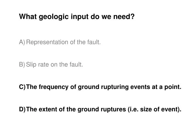
What geologic input do we need? Representation of the fault. Slip rate on the fault. The frequency of ground rupturing events at a point. The extent of the ground ruptures (i.e. size of event). The frequency of ground rupturing events at a point. Can be determined by:

E N D
What geologic input do we need? • Representation of the fault. • Slip rate on the fault. • The frequency of ground rupturing events at a point. • The extent of the ground ruptures (i.e. size of event).
The frequency of ground rupturing events at a point. • Can be determined by: • Dated series of paleo-earthquakes • Average slip per event (divided by slip rate) • Slip during a historic event (assume it is average and divided by slip rate). • Scaling relationships (infer slip per event from fault or segment length and divide by slip rate). • Assume it behaves like similar or adjacent faults or segments. • Infer from the open historical interval. • Guess • ………
The extent of the ground ruptures (i.e. size of event). Once we know the recurrence interval for each piece (segment) we need to decide the extent of each earthquake. We can look at the extent of historic events or steps in displacement along historic events. We can use the similarity of timing between individual events on adjacent segments, or the lack of agreement to limit rupture extent. We can use the similarity/difference between the number of events in a time interval between adjacent segments. We can use the size of the displacement, assuming that large displacement are likely to extend farther, or that similar displacements on adjacent segments imply continuity, etc.
The Geologic Insight model falls between the maximum and minimum earthquakes models. Given that the segmentation and RIs are correct we believe that the maximum and minimum earthquakes models span the likely range of possibilities. For large, mature faults like the San Andreas the geologic insight model is usually closer to the minimum earthquakes model. For smaller and less integrated faults the geologic insight is closer to the maximum earthquakes model.
Although not called maximum and minimum earthquakes models, the 02 Bay Area Working Group included models with the maximum and minimum number of possible earthquakes. The big difference is that each of their models included a mix of what we would call geologic insight, max, and min, whereas we have separated them.
Let’s focus on the Southern San Andreas fault • We examined the existing segmentation and concluded that we needed more segments to describe all possible ruptures (not to mention slip rate and geometry changes). • We generated maximum and minimum number of rupture models using the rules defined for all A-faults. • We attempted to quantify the geologic insight that goes into building geologic insight models. • We modified the quantitative results to be consistent with additional A-fault rules that we could not quantify.
Let’s focus on the Southern San Andreas fault • We examined the existing segmentation and concluded that we needed more segments to describe all possible ruptures. • We generated maximum and minimum number of rupture models using the rules defined for all A-faults. • We attempted to quantify the geologic insight that goes into building geologic insight models. • We modified the quantitative results to be consistent with additional A-fault rules that we could not quantify. • Let’s start with the Min and Max models.
Perhaps ironically the evidence for max and min earthquakes models is the same. If we plot all of the pdfs for all earthquakes on the southern San Andreas we find that most overlap at relatively narrow intervals of time. [Each color is a different site.] This means that large portions of the fault rupture together or that a series of smaller events propagate along the fault over a relatively short period of time. While some have questioned our maximum earthquakes model, it has happened on other faults, including the North Anatolian and Xianshuihe faults in this century. See Weldon et al., Science, 2005, for details and references to data sources.
Clearly we need more than just the age overlap to tell us rupture extents. In our geologic insight model, our goal is to somehow examine all possible combinations that the data permit, and rank or weight them by additional constraints.
We can also use The number of earthquakes in a scenario as one way of ranking scenarios. The lack of a southern SAF earthquake since 1857 constrains the probable number of ruptures in viable scenarios. E.g., 15 rupture scenarios are twice as likely as 22 rupture scenarios.
The extent of the ground ruptures (i.e. size of event). Once we know the recurrence interval for each piece (segment) we need to decide the extent of each earthquake. We can look at the extent of historic events or steps in displacement along historic events. We can use the similarity of timing between individual events on adjacent segments, or the lack of agreement to limit rupture extent. We can use the similarity/difference between the number of events in a time interval between adjacent segments. We can use the size of the displacement, assuming that large displacement are likely to extend farther, or that similar displacements on adjacent segments imply continuity, etc.
Constrained Probability Model 2_1 Segmented, Fewest ruptures from limited set Chol Carr BBnd MojN MojS NSBr SSBr SGor Coac Pkfl 0.010 0.010 0.209 0.010 0.540 0.139 0.052 0.010 0.010 Chol 0.010 0.256 0.037 0.010 0.621 0.037 0.010 0.010 0.010 Carr 0.000 0.056 0.010 0.010 0.621 0.113 0.169 0.010 0.010 BBnd 0.000 0.000 0.010 0.010 0.277 0.010 0.416 0.139 0.139 MojN 0.000 0.000 0.000 0.010 0.457 0.038 0.381 0.076 0.038 MojS 0.000 0.000 0.000 0.000 0.495 0.148 0.297 0.010 0.050 NSBr 0.000 0.000 0.000 0.000 0.000 0.346 0.271 0.098 0.286 SSBr 0.000 0.000 0.000 0.000 0.000 0.000 0.735 0.010 0.255 SGor 0.000 0.000 0.000 0.000 0.000 0.000 0.000 0.722 0.278 Coac 0.000 0.000 0.000 0.000 0.000 0.000 0.000 0.000 1.000 Constrained Probability Model 2_1 Segmented, Best Displacements from limited set Chol Carr BBnd MojN MojS NSBr SSBr SGor Coac Pkfl 0.010 0.010 0.163 0.010 0.718 0.049 0.010 0.010 0.010 Chol 0.010 0.250 0.083 0.010 0.543 0.042 0.042 0.010 0.010 Carr 0.000 0.240 0.010 0.010 0.540 0.120 0.060 0.010 0.010 BBnd 0.000 0.000 0.010 0.010 0.679 0.010 0.010 0.271 0.010 MojN 0.000 0.000 0.000 0.010 0.398 0.092 0.306 0.184 0.010 MojS 0.000 0.000 0.000 0.000 0.742 0.062 0.124 0.062 0.010 NSBr 0.000 0.000 0.000 0.000 0.000 0.370 0.344 0.117 0.169 SSBr 0.000 0.000 0.000 0.000 0.000 0.000 0.881 0.024 0.095 SGor 0.000 0.000 0.000 0.000 0.000 0.000 0.000 0.545 0.455 Coac 0.000 0.000 0.000 0.000 0.000 0.000 0.000 0.000 1.000
<7.1 7.1-7.4 7.4-7.7 7.7-8.0 >8.0 total types CH (02)M1 21.5 0.0 13.8 13.8 14.2 63.2 3 CH (02)M2 0.0 25.0 0.0 47.2 0.0 72.2 2 CH (02)M3 23.7 0.0 0.0 63.2 0.0 86.9 2 CH WG07 20.0 2.5 12.5 28.0 4.5 67.5 18 CC (02)M1 0.0 6.3 20.0 13.8 14.2 54.2 4 CC (02)M2 0.0 0.0 0.0 47.2 0.0 47.2 1 CC (02)M3 0.0 9.3 9.3 63.2 0.0 81.8 2 CC WG07 3.5 4.0 16.3 36.3 4.5 64.5 31 MJ (02)M1 0.0 13.1 0.0 32.6 14.2 59.9 3 MJ (02)M2 0.0 10.3 10.3 47.2 0.0 67.7 2 MJ (02)M3 0.0 13.9 0.0 63.2 0.0 77.1 2 MJ WG07 0.5 5.0 22.8 50.8 4.5 83.5 35 SB (02)M1 0.0 0.0 7.7 32.6 14.2 54.5 3 SB (02)M2 0.0 0.0 27.4 27.4 0.0 54.8 1 SB (02)M3 0.0 0.0 47.8 33.8 0.0 81.6 2 SB WG07 7.3 8.5 20.5 34.8 4.5 75.5 33 CO (02)M1 0.0 11.5 0.0 32.6 14.2 58.3 3 CO (02)M2 0.0 0.0 27.4 27.4 0.0 54.8 1 CO (02)M3 0.0 13.0 33.8 33.8 0.0 80.5 2 CO WG07 20.0 3.5 8.0 12.5 4.5 48.5 10