Download
1 / 33
340 likes | 506 Views
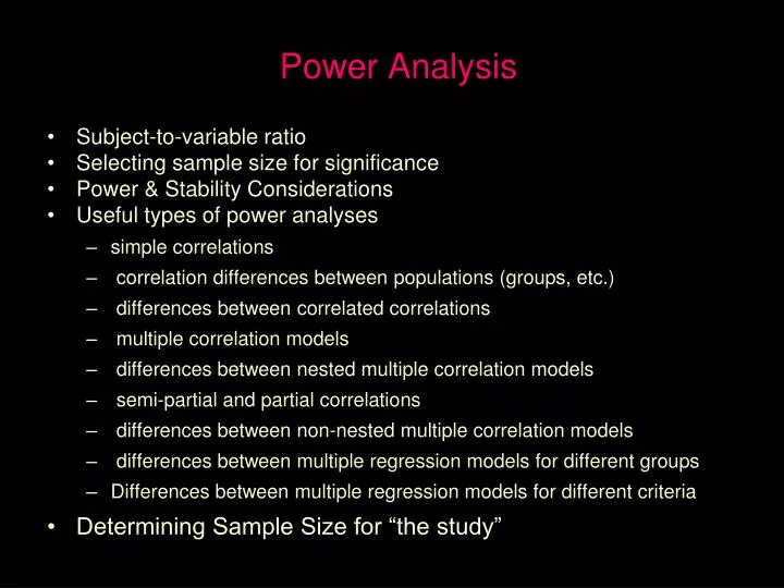
Power Analysis. Subject-to-variable ratio Selecting sample size for significance Power & Stability Considerations Useful types of power analyses simple correlations correlation differences between populations (groups, etc.) differences between correlated correlations

E N D
Power Analysis • Subject-to-variable ratio • Selecting sample size for significance • Power & Stability Considerations • Useful types of power analyses • simple correlations • correlation differences between populations (groups, etc.) • differences between correlated correlations • multiple correlation models • differences between nested multiple correlation models • semi-partial and partial correlations • differences between non-nested multiple correlation models • differences between multiple regression models for different groups • Differences between multiple regression models for different criteria • Determining Sample Size for “the study”
Sample Size & Multiple Regression • The general admonition that “larger samples are better” has considerable merit, but limited utility… • R² will always be 1.00 if k = N-1 (it’s a math thing) • R² will usually be“too large” if the sample size is “too small” (same principle but operating on a lesser scale) • R² will always be larger on the modeling sample than on any replication using the same regression weights • R² & b-values will replicate better or poorer, depending upon the stability of the correlation matrix values • R² & b-values of all predictors may vary with poor stability of any portion of the correlation matrix (any subset of predictors) • F- & t-test p-values will vary with the stability & power of the sample size – both modeling and replication samples
Subject-to-Variable Ratio • How many participants should we have for a given number of predictors? -- usually refers to the full model • The subject/variable ratio has been an attempt to ensure that the sample is “large enough” to minimize “parameter inflation” and improve “replicability”. • Here are some common admonitions.. • 20 participants per predictor • a minimum of 100 participants, plus 10 per predictor • 10 participants per predictor • 200 participants for up to k=10 predictors and 300 if k>10 • 1000 participants per predictor • a minimum of 2000 participants, + 1000 for each 5 predictors
As is often the case, different rules of thumb have grown out of different research traditions, for example… • chemistry, which works with very reliable measures and stable populations, calls for very small s/v ratios • biology, also working largely with “real measurements” (length, weight, behavioral counts) often calls for small s/v ratios • economics, fairly stable measures and very large (cheap) databases often calls for huge s/v ratios • education, often under considerable legal and political scrutiny, (data vary in quality) often calls for fairly large s/v ratios • psychology, with self-report measures of limited quality, but costly data-collection procedures, often “shaves” the s/v ratio a bit
Problems with Subject-to-variable ratio • #1 neither n, N nor N/k is used to compute R² or b-values • R² & b/-values are computed from the correlation matrix • N is used to compute the significance test of the R² & each b-weight • #2 Statistical Power Analyses involves more than N & k • We know from even rudimentary treatments of statistical power analysis that there are four attributes of a statistical test that are inextricably intertwined for the purposes of NHST… • acceptable Type I error rate (chance of a “false alarm”) • acceptable Type II error rate (chance of a “miss”) • size of the effect being tested for • sample size We will “forsake” the subjects-to-variables ratio for more formal power analyses & also consider the stability of parameter estimates (especially when we expect large effect sizes).
“Selecting S for significance” • estimate the pairwise effect size, say r = .35 • using the correlation critical-value table, select a sample size for which that effect size will be significant • r = .35 will be significant if df = 30 or S=32 Partial critical-r Table df = .05 20 .42 25 .38 30 .35 35 .33 40 .30 45 .29 50 .27 60 .25 What’s the power of this sample size ?? For r = .35 & S=30, Power is only 50% So, this approach leads to very low power !
Why do these two approaches differ so much ? The difference in “suggested S” is because the power analysis takes into account that the r-value of a sample drawn from a population with r = .361 might, by chance, be smaller than .361 !!! Remember that we are testing RH: and making inferences about the population correlation !!!! So, we want to be able to correctly decide that there is a correlation in the population (i.e., reject H0:), even if the sample we happen to draw has a smaller r-value than the population. By the way… For a given r the sample size for 80% power is about 2X the sample size for which that r will be significant (p = .05)
NHST Power “vs.” Parameter estimate stability • NHST power what’s the chances of rejecting a “false null” vs. making a Type II error? • Statistical power is based on… • size of the effect involved (“larger effects are easier to find”) • amount of power (probability of rejecting H0: if effect size is as expected or larger) • Stability how much error is there in the sample-based estimate of a parameter (correlation, regression weight, etc.) ? • Stability is based on … • “quality” of the sample (sampling process & attrition) • sample size • Std of r = 1 / (N-3), so … • N=50 r +/- .146 N=100 r +/- .101 N=200 r +/- .07 • N=300 r +/- .058 N=500 r +/- .045 N=1000 r +/- .031
The power table only tells us the sample size we need to reject H0: r=0!! It does not tell us the sample size we need to have a good estimate of the population r !!!!! Partial Power Table (taken & extrapolated from Friedman, 1982) r .15 .20 .25 .30 .35 .40 .45 .50 .55 .60 .65 .70 power .30 93 53 34 24 18 14 11 9 8 7 6 5 .40 132 74 47 33 24 19 15 12 10 8 7 6 .50 170 95 60 42 30 23 18 14 12 9 8 7 .60 257 143 90 62 45 34 24 20 16 13 11 9 .70 300 167 105 72 52 39 29 23 18 15 12 10 .80 343 191 120 82 59 44 33 26 20 16 13 11 .90 459 255 160 109 78 58 44 34 27 21 17 13 “Sufficient power” but “poor stability” • How can a sample have “sufficient power” but “poor stability”? • Notice it happens for large effect sizes!! • e.g., For a population with r = .30 & a sample of 100 … • Poor stability of r estimate +/- 1 std is .20-.40 • Large enough to reject H0: that r = 0 power almost .90
We know from even rudimentary treatments of statistical power analysis that there are four attributes of a statistical test that drive the issue of selecting the sample size needed a particular analysis… • acceptable Type I error rate (chance of a “false alarm”) • acceptable Type II error rate (chance of a “miss”) • size of the effect being tested for (.1=small, .3=med, .5=large) • sample size for that analysis We also know that power is not the only basis for determining “N” The stability/variability of each r in thecorrelation matrix is related to N Std of r = 1 / (N-3), so … N=50 r +/- .146 N=100 r +/- .101 N=200 r +/- .07 N=300 r +/- .058 N=500 r +/- .045 N=1000 r +/- .031
Power Analysis for Simple Correlation Post hoc I found r (22) = .30, p > .05, what’s the chance I made a Type II error ?? N = Power = Chance Type II error A priori #1 I expect my correlation will be about .25, & want power = .90 sample size should be = #2 Expect correlations of .30, .45, and .20 from my three predictors & want power = .80 sample size should be = 24 .30 .70 160 191, based on lowest r = .20
Power Analysis for Simple Correlation On the following page is a copy of the power analysis table from the first portion of the course. Some practice... Post hoc I found r (22) = .30, p < .05, what’s the chance I made a Type II error ?? N = Power = Chance Type II error A priori #1 I expect my correlation will be about .25, & want power = .90 sample size should be = #2 Expect correlations of .30, .45, and .20 from my three predictors & want power = .80 sample size should be = 24 .30 .70 160 191, based on lowest r = .20
Putting Stability & Power together to determine the sample size 1. Start with stability – remember … Std of r = 1 / (N-3), so … N=50 r +/- .146 N=100 r +/- .101 N=200 r +/- .07 N=300 r +/- .058 N=500 r +/- .045 N=1000 r +/- .031 … suggesting that 200-300 is a good guess for most analyses (but more is better). 2. Then for the specific analysis, do the power analysis … For the expected r/R² & desired power, what is the required sample size? 3. Use the larger of the stability & power estimates !
An example …. We expect a correlation of .60, and want only a 10% risk of a Type II error if that is the population correlation Looking at the power table for r = .60 and power = .90.. … the suggested sample size is 21 N = 21, means the std of the correlation estimates (if we took multiple samples from the target population is 1 / (21-3) = .35 With N = 21 we’ve a 90% chance of getting a correlation large enough to reject the Null on average, our estimate of the population correlation will be wrong my .35. We’d certainly interpret a .25 and a .95 differently In this case we’d go with the 200-300 estimate, in order to have sufficient stability – we’ll have lots of power!
Another example …. We expect a correlation of .10, and want only a 20% risk of a Type II error if that is the population correlation Considering stability – let’s say we decide to go with 300 Looking at the power table for r = .10 and power = .80.. … the suggested sample size is 781 With N = 300, we’d only have power of about .40 … 60% chance of a Type II error. In this case we’d go with the 781 estimate (if we can afford it), in order to have sufficient power – we’ll have great stability of +/- .036 !
Power analysis for correlation differences between populations • the Bad News • this is a very weak test -- requires roughly 2x the N to test for a particular r-r value than to test for a comparable r-value • the Good News • the test is commonly used, well-understood and tables have been constructed for our enjoyment (from Cohen, 1988) • Important! Decide if you are comparing r or |r| values • r1 - r2 .10 .20 .30 .40 .50 .60 .70 .80 • Power • .25 333 86 40 24 16 12 10 8 • .50 771 195 88 51 34 24 19 15 • .70 1237 333 140 89 52 37 28 22 • .80 1573 395 177 101 66 47 35 28 • .90 2602 653 292 165 107 75 56 44 • all values for = .05 Values are “S” which is total sample size
Power Analysis for Comparing “Correlated Correlations” • It takes much more power to test the H0: about correlations differences than to test the H0: about each r = .00 • Most discussions of power analysis don’t include this model • Some sources suggest using the tables designed for comparing correlations across populations (Fisher’s Z-test) • Other sources suggest using twice the sample size one would use if looking for r = the expected r-difference (works out to about the same thing as above suggestion) • Each of these depends upon having a good estimate of both correlations, so that the estimate of the correlation difference is reasonably accurate • It can be informative to consider the necessary sample sizes for differences in the estimates of each correlation
Here’s an example … • Suppose you want to compare the correlations of GREQ and GREA with graduate school performance. • Based on a review of the literature, you expect that… • GREQ and grad performance will correlate about .4 • GREA and grad performance will correlate about .6 • so you would use the value of r-r = .20 … • and get the estimated necessary sample size of N = 395 • To consider how important are the estimates of r… • if the correlations were .35 and .65, then with r-r = .30, N= 177 • if the correlations were .45 and .55, the with r-r=.10, N= 1573
Power Analysis for Multiple regression Power analysis for multiple regression is about the same as for simple regression, we decide on values for some parameters and then we consult a table … Remember the F-test of H0: R² = 0 ?? R² / k R² N-k-1 F = -------------------- = ---------- * --------- 1-R² / N - k - 1 1 - R² k Which corresponds to: significance test = effect size * sample size So, our power analysis will be based not on R² per se, but on the power of the F-test of the H0: R² = 0
Using the power tables (post hoc) for multiple regression (single model) requires that we have four values: a = the p-value we want to use (usually .05) u = df associated with the model ( we’ve used “k”) v = df associated with F-test error term (N - u - 1) f² =(effect size estimate)= R² / (1 - R²) = f² * ( u + v + 1) This is the basis for determining power E.g., N = 96, and 5 predictors, R² = .10 was found a = .05 u = 5 v = 96 - 5 - 1 = 90 f² = .1 / (1 - .1) = .1111 = .1111 * (5 + 89 + 1) = 10.6 Go to table -- a = .05, & u = 5 = 10 12 v = 6063 72 power is around .68 12065 75
Another N = 48, and 6 predictors, R² = .20 (p < .05) a = u = v = f² = = Go to table -- a = .05&u = 6 = 12 v = 20 power is about 60 This sort of post hoc power analysis is, as before, especially helpful when the H0: has been retained -- to determine whether the result is likely to have been a Type II error. Remember that one has to decide how small of an effect is “meaningful”, and adjust the sample size to that decision. .05 6 .2 / (1 - .2) = .25 .25 * (6 + 41 + 1) = 12 59 68 .64
a priori power analyses for multiple regression are complicated by ... • Use of (combo of effect & sample size) rather than R² (just the effect size) in the table. • This means that sample size enters into the process TWICE • when computing = f² * ( u + v + 1) • when picking the “v” row to use v = N - u - 1 • So, so the of an analysis reflects the combination of the effect size and sample size, which then has differential power depending (again) upon sample size (v). • E.g.#1, R² = .20 f² = .2 / (1-.2) = .25 N = 50 = .25 * ( 50) =12.5 with u = 10, and v = N - 10 - 1 = 39 --power is about .50 • E.g.#2, R² = .40 f² = .4 / (1 - .4) = .67 N = 19 = .67 * (19) = 12.5 with u = 10, and v = 19 - 19 - 1 = 8 --power is about .22 • So, for a priori analyses, we need the sample size estimate to compute the to use to look up the sample size estimate we need for a given level of statistical power ????
Perhaps the easiest way to do a priori sample size estimation is to play the “what if game” . . . I expect that my 4-predictor model will account for about 12% of the variance in the criterion -- what sample size should I use ??? a = .05 u= 4 f² = R² / (1 - R²) =.12 / (1 - .12) = .136 “what if..” N = 25 N = 65 N = 125v= (N - u - 1) = 20 60 120 = f² * ( u + v + 1) = 3.4 8.8 17.0 Using the table… power = about .21 about .62 about .915 If we were looking for power of .80, we might then try N = 95 so v = 90, = 12.2, power = about .77(I’d go with N = 100-110)
Power Analysis for comparing nested multiple regression models (R²)… The good news is that this process is almost the same as was the power analysis for R². Now we need the power of … R²L - R²S / kL - ks R²L - R²S N - kl - 1 F = -------------------------- = --------------- * ------------ 1 - R²L / N - kl - 1 1 - R²L kL - ks Which, once again, corresponds to: significance test = effect size * sample size the notation we’ll use is … R2Y-A,B - R2Y-A -- testing the contribution of the “B” set of variables
Using the power tables (post hoc) for R² (comparing nested models) requires that we have four values: a = the p-value we want to use (usually .05) w = # predictors different between the two models) u= # predictors associated with the smaller model v = df associated with F-test error term (N - u - w - 1) f² = (effect size estimate) = (R²L - R²S) / (1 - R²L) = f² * ( u + v + 1) , where Post Hoc E.g.,N = 65, R²L (k=5) = .35, R²S (k=3) = .15 a = .05 w = 2 u = 3 v = 65 - 2 - 3 - 1 = 59 f² = .35 - .15 / 1 - .35 = .3077 = .3077 * (3 + 59 + 1) = 19.4 Go to table -- a = .05 & u = 3 = 20 power about .97 v = 60.97
a priori power analyses for nested model comparisons are probably most easily done using the “what if “ approach I expect that my 4-predictor model will account for about 12% of the variance in the criterion and that including an additional 3 variables will increase the R² to about .18 -- what sample size should I use ??? a = .05 w = 3 u= 4 f² = (RL² - RS²) / (1 - R²) =(.18 - .12) / (1 - .18) = .073 “what if..” N = 28 N = 68 N = 128N = 208 () v= (N - u - w - 1) = 20 60 120 200 () = f² * ( u + v + 1) = 1.83 4.75 9.13 15.0 Using the table… power = < .15 about .37 about .64 about .89 If we were looking for power of .80, we might then try N = 158 so v = 150, = 11.3 power = about .77(I’d go with N = 180 or so)
Power Analysis for Semi-partial Correlations A semi-partial correlation can be obtained from the difference between two multiple regression models… rY(,A.B) = √ R²Y.AB - R²Y.B or … … the correlation between Y & A, controlling A for B, is the square root of the unique contribution of A to the A-B model So,we could perform power analyses for semi-partial correlations using the same process we use for a nested model comparison. Now we need the power of … R²Y.AB - R²Y.B F = ------------------------------ 1 - R²Y.AB / N - kL – 1 note: kL – kS = 1 While simple to calculate, the difficulty with this approach is that we need to know not only the expected value of the semi-partial, but also of the related multiple R2 – something that we rarely have! For this reason, the common (and workable) way to estimate sample size for a semi-partial correlation is to use the power table for a simple correlation
Power Analysis for Multiple Semi-partial Correlations Any semi-partial or multiple semi-partial uses the same idea … rY(,A.B,C,D) = √ R²Y.ABCD - R²Y.BCD or … … the correlation between Y & A, controlling A for B, C & D, is the square root of the unique contribution of A to the ABCD model So,we perform power analyses for semi-partial correlations using the same process we use for a nested model comparison. Now we need the power of … R²Y.ABCD - R²Y.BCD F = -------------------------------------- 1 - R²Y.ABCD / N - kL – 1 This has the same problem as a estimating power for a semi-partial, with the same solution – use correlation power table as an estimate of a proper sample size.
Power Analysis for Partial Correlations A partial correlation can be obtained from the difference between two multiple regression models (re-scaled a bit) … √ R²Y.AB - R²Y.B r Y(,A.B) = ------------------------ 1 - R²Y.B So, we perform power analyses for partial correlations using the same process we use for a nested model comparison. Now we need the power of … R²Y.AB - R²Y.B F = ------------------------------ 1 - R²Y.AB / N - kL – 1 note: kL – kS = 1 This has the same problem as a estimating power for a semi-partial, with the same solution – use correlation power table as an estimate of the proper sample size
Testing non-nested multiple regression models… • It is essentially the same process as you used earlier for comparing “correlated correlations”… • What we will do is… • estimate each of the correlation values • R for the one model • R for the other model • find R-R and apply the Fisher’s Z-test power table
Comparing multiple regression models across groups Remember, there are two portions of this comparison – we need to do the power for each 1. Comparing how well the predictors “work” for the two groups -- estimate Rg1-Rg2 and apply the Fisher’s Z-test power table 2. Comparing the “structure” of the model from the 2 groups -- estimate Rdirect – Rcross and apply the Fisher’s power table (this is an approximation, as was using this table for correlated correlations earlier)
Comparing multiple regression models across criteria Comparing the “structure” of the model from the 2 criteria -- estimate Rdirect – Rcross and apply the Fisher’s power table (this is an approximation, as was using this table for correlated correlations earlier) Notice how blythly we say we will estimate all of these R-values in these last two types of power analyses. Often we can’t estimate them well, and should play the “what-if” game to consider what power we will have for different possibilities!!!
Considering the sample size for the Study Really a simple process, but sometimes the answer is daunting! First: For each analysis (r or R²) perform the power analysis consider the “200-300” suggestion & resulting stability pick the larger value as the N estimate for that analysis Then: Looking at the set of N estimates for all the analyses … The largest estimate is the best bet for the study This means we will base our study sample size on the sample size required for the least powerful significance test ! Usually this is the smallest simple correlation or a small R² with a large number of predictors.