Download
1 / 14
140 likes | 249 Views
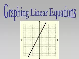
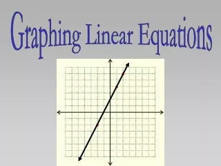
Graphing Linear Equations. Unit 5.08. I can graph linear equations in slope-intercept form. I can also identify and interpret the unit rate and starting point from a graph!. Put it all together!. Unit Rate. Constant Rate of Change. Change in y Change in x. Rise Run. SLOPE!.

E N D
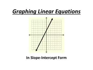
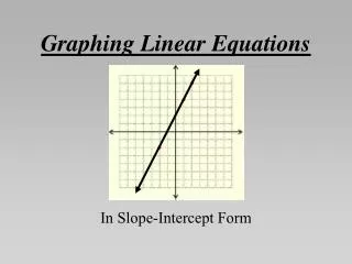
Graphing Linear Equations Unit 5.08 I can graph linear equations in slope-intercept form. I can also identify and interpret the unit rate and starting point from a graph!
Put it all together! Unit Rate Constant Rate of Change Change in y Change in x Rise Run SLOPE!
Vocabulary Slope:The“rise over run”, describes the steepness of a line. In mathematics, we use the variable m to represent slope.
Put it all together! Starting Point Y-Intercept!
Vocabulary Slope:The“Rise over Run”, describes the steepness of a line. In mathematics, we use the variable m to represent slope. Y-Intercept:Where the graph of a line crosses the y-axis. In mathematics, we use the variable b to represent the y-intercept.
Vocabulary (Review) Slope Intercept Form:A linear equation written in the form y = mx + b. dd * The slope (or unit rate) of the line is m. * The y-intercept (or starting point) is b. Example: In the equation y = ½x + 3, the slope is½and the y-intercept is3. Let’s graph this equation!
1) y = mx + b Step 1: If we know that the y-intercept (starting point) is 3, then we can plot the point (0, 3) on the graph. Step 2: From that point, we count the “rise over run” (unit rate) of the slope to find other points on the line. Step 3: Connect the dots.
2) y = mx + b Step 1: If we know that the y-intercept (starting point) is -5, then we can plot the point (0, -5) on the graph. Step 2: From that point, we count the “rise over run” (unit rate) of the slope to find other points on the line. Step 3: Connect the dots.
3) y = mx + b Step 1: If we know that the y-intercept (starting point) is 0, then we can plot the point (0, 0) on the origin of the graph. Step 2: From that point, we count the “rise over run” (unit rate) of the slope to find other points on the line. Step 3: Connect the dots.
The examples so far have all had positive slope. What would the graph of a line with negative slope look like?
4) y = mx + b Step 1: If we know that the y-intercept (starting point) is 2, then we can plot the point (0, 2) on the graph. Step 2: From that point, we count the “rise over run” (unit rate) of the slope to find other points on the line. Step 3: Connect the dots.
5) y = mx + b Step 1: If we know that the y-intercept (starting point) is 6, then we can plot the point (0, 6) on the graph. Step 2: From that point, we count the “rise over run” (unit rate) of the slope to find other points on the line. Step 3: Connect the dots.
Try These! 6) 7)
Homework Time! 5.08 Graphing Linear Equations WS I can graph linear equations in slope-intercept form. I can also identify and interpret the unit rate and starting point from a graph!