Download
1 / 27
270 likes | 517 Views
Participating Media Illumination using Light Propagation Maps. Raanan Fattal Hebrew University of Jerusalem, Israel. Introduction. In media like fog, smoke and marble light is: Scattered Absorbed Emitted Realistic rendering by accounting such phenomena. Images by H. W. Jensen.

E N D
Participating Media Illumination using Light Propagation Maps Raanan Fattal Hebrew University of Jerusalem, Israel
Introduction • In media like fog, smoke and marble light is: • Scattered • Absorbed • Emitted • Realistic rendering by accounting such phenomena Images by H. W. Jensen
Introduction • The Radiative Transport Eqn. models these events I(x,w) – radiation intensity (W/m2sr) emission absorption out-scattering change along w in-scattering
Solving the RTE – Previous Work • In 3D, the RTE involves 5-dimensional variables, • Much work put into calculating the solution • Common approaches are: • volume-to-volume energy exchange • stochastic path tracing • Discrete Ordinates methods • Methods survey [Perez, Pueyo, and Sillion 1997]
Previous Work • The Zonal Method[Hottel & Sarofim 1967, Rushmeier 1988] • Compute exchange factor between every volume pair • In 3D , involves O(n7/3) relations for isotropic scattering • Hierarchical clustering strategy [Sillion 1995]reduce complexity
Previous Work • Monte Carlo Methods: • Photon tracing techniques [Pattanaiket al. 1993, Jensen et al. 1998] • Path tracing techniques [Lafortuneet al. 1996] • Light particles are tracked within the media • Noise requires many paths per a pixel • Unique motion many computations per a photon Pattanaiket al. 1993 Jensen et al. 1998 Lafortuneet al. 1996
Previous Work • Discrete Ordinates[Chandrasekhar 60, Liu and Pollard 96 , Jessee and Fiveland 97, Coelho 02,04] • Both space and orientation are discretized • Derive discrete eqns. and solve • The DOM suffers two error types cell volume angular index spatial indices Discrete light directions inside a spatial voxel
Discrete Ordinates • ‘Numerical smearing’ (or ‘false scattering’) • Discrete flux approx. involves successive interpolations • smear intensity profile or • generate oscillations • Analog of numerical dissipation/diffusion in CFD (showing ray’s cross section) 1st order 2nd order
Discrete Ordinates • ‘Ray effect’ • Light propagates in (finite) discrete directions • Spurious light streaks from concentrated light areas • New method can be viewed as a form of DOM Jet color scheme
New Method - Overview • Iterative solvers Progressive Radiosity & Zonal propagate light [Gortleret al. 94] Idea: propagate light using 2D Light Propagation Maps (LPM) and not use DOM eqns. in 3D stationary grid • One physical dimension less • Partial set of directions stored • Allow higher angular resolution • Unattached to stationary grid • Advected parametrically stationary grid Offer a practical remedy to the ‘ray effect’ No interpolations needed for light flux, ‘false scattering’ is eliminated Light Propagation Maps, 2D grids of rays, each covering different set of directions
New Method - Setup • Variables: • average scattered light (unlike DOM) • (need only 1 angular bin for isotropic scattering!) • - ray’s intensity • - ray’s position • Goal: compute stationary grid light propagation map LPM 2D indexing
New Method - Derivation • Next: derive the eqns. for and their relation to Plug in L instead of I, and R – ray’s pos. instead of x Approx. using discrete fields (zero order) Note: in the in-scattering term, I wasn’t replaced by L Introduce an unpropagated light field U instead of sources stationary grid single light ray in LPM
New Method - Derivation • As done in Progressive Radiosity, the solution • is constructed by accumulating light from LPMs • (A -discrete surface areas, F – phase func. weights) • This is also added to the unpropagated light field U I(x,w)=
New Method – an Iteration • Rays integrate U – emptying relevant bins • LPM ray’s dirs. must be included in U’s • Coarse bins of I, U contain scattered light, filtered by phase func. • Linear light motion: inadequate to simulate Caustics • Light scattered from rays added to U, I stationary grid • Proceed to next layer - repeat • Sweep along other directions (6 in 3D)
Results DOM with 54 angular bins o o o o o o o o o For 643 with 9x9x6=54 angular bins DOM requires 510MBs Using LPM of 9x9 requires < 1MB and grid 6MB LPM 9x9 angles in LPM, 1+6 in grid Less memory for stationary grid!
Results DOM with 54 ordinates on 1283 spurious light ray 9x9 ordinates in LPM on 1283 Same coarse grid res. (6 dirs. isotropic sct.)
Results First-order upwind Second-order upwind High-res. 2nd-order upwind LPM parametric advection
Results Comparison with Monte Carlo MC with 5x10⁶ particles, 17.6 mins MC with 106 particles, 3.5 mins. 9x9 LPM,3.7 mins
Results – Clouds Scenes Back lit Top lit
Results - Marble Constant scattering Perturbed absorption (isotropic, 52x1283) Perturbed scattering Zero absorption (isotropic, 52x1283)
Results – Two “wavelengths” Two simulations combined (isotropic, 52x1283)
Results Hygia, Model courtesy of: Image-based 3D Models Archive, Telecom Paris (isotropic, 52x2563)
Results - Smoke CFD smoke animation (isotropic, 72x643)
Summary • Running times (3 scat. generations x 6 sweeps): • 643 (isotropic), LPM of 5x5 – 17 seconds • 643 (isotropic), LPM of 9x9 – 125 seconds • 643 3x3(x6), LPM of 6x6 – 60 seconds (2.7 GHz Pentium IV) • Light rays advected collectively and independently • Avoids grid truncation errors - No numerical smearing • Less memory more ordinates – Reduced ray effect
Results • In scenes with variable s, indirect light travels straight
Discrete Ordinates • In CFD, advected flux is treated via Flux Limiters • high-order stencils on smooth regions • switch to low-order near discontinuities • For the RTE such ‘High res.’ methods suffer from: • still, some amount of initial smearing is produced • limiters are not linear, yielding a non-linear system of eqns. • offers no remedy to the ‘ray effect’ discussed next