Download
1 / 36
420 likes | 630 Views
Computer Graphics Global Illumination: Photon Mapping , Participating Media Lecture 1 2 Taku Komura. last lecture . Monte-Carlo Ray Tracing Path Tracing Bidirectional Path Tracing Photon Mapping. Today. Methods to accelerate the accuracy of photon mapping

E N D
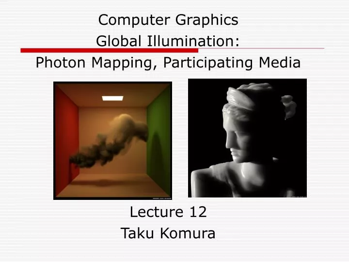
Computer Graphics Global Illumination: Photon Mapping, Participating Media Lecture 12 Taku Komura
last lecture • Monte-Carlo Ray Tracing • Path Tracing • Bidirectional Path Tracing • Photon Mapping
Today • Methods to accelerate the accuracy of photon mapping • Rendering Participating Media
Accelerating the accuracy of photon mapping • Combine with ray tracing to visualize the specular light visible from the camera • Shoot more photons towards directions where more samples are needed • Caustics photon map • Tracing photons only towards specular surfaces
A Practical Two-Pass Algorithm • Building photon maps by photon tracing • Separate the photon paths into different categories according to the reflectance • Rendering • Combining the radiance of difference light paths
Light Transport Notation • L: Lightsource • E: Eye • S: Specular reflection • D: Diffuse reflection • (k)+ one or more k events • (k)* zero or more of k events • (k)? zero or one k event • (k|k’) a k or k’ event
Photon Tracing • Create two photon maps • Global photon map (the usual photon map) • All Photons with property L(S|D)*D are stored. • Caustics photon map • Created by tracing photons that hit the specular surfaces • Cast the photons only toward specular objects • LS+D
Rendering • Separate the irradiance into four groups • Direct illumination (by ray tracing or global photon map) : LD • Diffuse indirect illumination (by global photon map) : LD(S|D)+D • Specular reflection (by ray tracing) L(S|D)*S • Caustics (by caustics photon map)LS+D
Caustics Photon Map • Caustics require high resolution • Need to cast more photons towards surfaces that generates caustics • Projection Map
Projection map • A map of the geometry seen from the light source • Made of many cells – which is on if there is a geometry in that direction, and off if not • For a point light, it is a spherical projection • For directional light, a planar projection • Use a bounding sphere to represent the objects
Why is photon mapping efficient? • It is a stochastic approach that estimates the radiance from a few number of samples • Kernel density estimation • Can actively distribute samples to important areas • Caustics photon map
Today • Methods to accelerate the accuracy of photon mapping • Rendering Participating Media
Participating Media • Dusty air, clouds, silky water • Translucent materials such as marble, skin, and plants • Photon mapping is good in handling participating media • In participating media, the light is scattered to different directions
The brightness of a point • Is decided by • Out scattering • Absorption • In scattering
Light out-scattering • The change in radiance, L, in the direction ω, due to out scattering is given by • The change in radiance due to absorption is
In-scattering • The change due to inscattering where the incident radiance, Li, is integrated over all directions p is called the phase function describing the distribution of the scattered light
Phase function • Isotropic scattering • Scattered in any random direction • Henyey-Greenstein Phase Function • Scattered in the direction more towards the front • Dust, stone, clouds
Examples Cornell Box scene – isotropic, homogeneous participating medium. 200,000 photons used with 65,000 in the volume map. Radiance estimate used 100 photons. Cornell Box scene – anisotropic, homogeneous participating medium. 200,000 photons used with 65,000 in the volume map. Radiance estimate used 50 photons.
Ray marching and single scattering • Now we compute how the light will be accumulated along a ray • This is called ray marching where N is the number of light sources and Li is the radiance from each light source The last term is the light entering from behind, which is attenuated by proceeding Δx
Ray marching through a finite size medium (Single Scattering)
Multiple scattering • For multiple scattering, it is necessary to integrate all the in-scattered radiance at every segment • Here S sample rays are used to estimate the in-scattered light
Photon mapping participating media • Photon mapping can efficiently handle multiple scattering • The photons interact with the media and are scattered / absorbed • The average distance the photon proceeds after each interaction is • Here S sample rays are used to estimate the in-scattered light
Photon Scattering • The photon is either absorbed or scattered • The probability of scattering is • Deciding what happens by Russian Roulette • Once the photon interacts with the media, it is stored in a volume photon map
Volume Radiance Estimate • Same as we did for surface radiance estimate, locate n nearest photons and estimate the radiance
Rendering Participating Media • By ray tracing • If a ray enters a participating media, we use ray marching to integrate the illumination. Single scattering term multiple scattering term
Examples single scattering multiple scattering
Subsurface Scattering • In computer graphics, reflections of non-metallic materials are usually approximated by diffuse reflections. • Light leaving from the same location where it enters the object • For translucent materials such as marble, skin and milk, this is a bad approximation • The light leaves from different locations
Single scattering • Direct single scattering: • Compute the distance the light has traveled and attenuate according to the distance • Indirect Multiple scattering : • Photon maps
Subsurface Scattering by Photon Mapping • Photon tracing – as explained before • Rendering – Ray marching
BSSRDF • Bidirectional Scattering Surface Reflectance Distribution Function (BSSRDF) • Relates the differential reflected radiance dLr, at x in the direction ω, to the differential incident flux, dΦ, at x’ from direction ω’. • We can capture/model the BSSRDF and use it for rendering
Rendering using BSSRDF (a) sampling a BRDF (b) sampling a BSSRDF • Collect samples of incoming rays over an area http://graphics.ucsd.edu/~henrik/animations/BSSRDF-SIGGRAPH-ET2001.avi
Rendering by BSSRDF • Human skin reflectance simulated by BRDF BSSRDF • Readings : Realistic Image Synthesis Using Photon Mapping by Henrik Wann Jensen, AK Peters Chapter 9, 10