Download
1 / 39
400 likes | 528 Views
Chapter 11 Graphical Methods. Introduction. “A picture is often better than several numerical analyses” Stand-alone procedure, or used in conjunction with other statistical techniques. Table 11.1 Example Data. What is the general shape of the distribution of the data?

E N D
Introduction • “A picture is often better than several numerical analyses” • Stand-alone procedure, or used in conjunction with other statistical techniques.
What is the general shape of the distribution of the data? • Is it close to the shape of a normal distribution, or is it markedly non-normal? • Are there any number that are noticeably larger or smaller than the rest of the numbers?
11.1 Histogram • A commonly used starting point in summarizing data is to put the data into classes and then to construct a histogram. • A histogram is a bar chart that shows the relative frequencies of observations in each of several classes. • Rule for determining the number of classes: • “Power of 2 rule”: for n observations, we would use a classes, where 2a-1 < n < 2a • Roundup a = lnn / ln 2 (=ROUNDUP(LN(100)/LN(2), 0) • a ~
11.2 Stem-and-Leaf Display • A stem-and-leaf display is one of the newer graphical techniques. • It is one of many techniques that are generally referred to as exploratory data analysis (EDA) methods. • A stem-and-leaf display provides the same information as a histogram, without losing the individual values
11.2 Stem-and-Leaf Display 3 2 134 6 2 578 13 3 0122334 17 3 5679 26 4 001122334 35 4 555667899 49 5 00111122223344 (15) 5 555666778888999 36 6 00112233444 25 6 556678899 16 7 01234 11 7 56689 6 8 1234 2 8 57
11.3 Dot Diagrams • Also called one-dimensional scatter plots. • It is simply a one-dimensional display in which a dot is used to represent each point. • The dot diagram portrays the relationship between the numbers. • Limitation: small number of data
11.3.1 Digidot Plot • Digidot plot is a combination of a time sequence plot and a stem-and-leaf display. • The order in the stem-and-leaf display is determined by the time sequence, not by numerical order.
11.3.1 Digidot Plot 232 6419 32 76 05
11.4 Boxplot • It is another exploratory data analysis (EDA) tool. • A boxplot is a graphic that presents the median, the first and third quartiles, and any outliers present in the sample. • The interquartile range (IQR) is the difference between the third and first quartile. This is the distance needed to span the middle half of the data. • The IQR is roughly 1.34 for normally distributed data
Creating a Boxplot • Compute the median and the first and third quartiles of the sample. Indicate these with horizontal lines. Draw vertical lines to complete the box. • Find the largest sample value that is no more than 1.5 IQR above the third quartile, and the smallest sample value that is not more than 1.5 IQR below the first quartile. Extend vertical lines (whiskers) from the quartile lines to these points. • Points more than 1.5 IQR above the third quartile, or more than 1.5 IQR below the first quartile are designated as outliers. Plot each outlier individually.
Notice there are no outliers in these data. Looking at the four pieces of the boxplot, we can tell that the sample values are comparatively densely packed between the median and the third quartile. The lower whisker is a bit longer than the upper one, indicating that the data has a slightly longer lower tail than an upper tail. The distance between the first quartile and the median is greater than the distance between the median and the third quartile. This boxplot suggests that the data are skewed to the left. Example cont.
Comparative Boxplots • Sometimes we want to compare between more than one sample. • We can place the boxplots of the two samples side-by-side. • This will allow us to compare how the medians differ between samples, as well as the first and third quartile. • It also tells us about the difference in spread between the two samples.
11.5 Normal Probability Plot • Most statistical procedures used in quality improvement work are based on the assumption that the population is approximately normally distributed. • Check the assumption of normality: • chi-square goodness-of-fit tests • Kolmogorov-Smirnov goodness-of-fit tests • Anderson-Darling tests • Shapiro-Wilk tests • Normal probability plot
Finding a Distribution Probability plots are a good way to determine an appropriate distribution. Here is the idea: Suppose we have a random sample X1,…,Xn. We first arrange the data in ascending order. Then assign evenly spaced values between 0 and 1 to each Xi. There are several acceptable ways to this; the simplest is to assign the value (i – 0.5)/n to Xi. The distribution that we are comparing the X’s to should have a mean and variance that match the sample mean and variance. We want to plot (Xi, F(Xi)), if this plot resembles the cdf of the distribution that we are interested in, then we conclude that that is the distribution the data came from.
11.6 Plotting Three Variables • Casement display: a set of two-variable scatter plots • If the 3rd variable is discrete, a scatter plot is produced for each value of that variable • If the 3rd variable is continuous, intervals for that variable would be constructed and the scatter plots then produced • Draftsman’s display: the set of three two-variable scatter plots arranged in a particular manner
11.6 Plotting Three Variables http://www.survo.fi/gallery/019.html
11.6 Plotting Three Variables http://www.mathworks.com/products/statistics/demos.html? file=/products/demos/shipping/stats/mvplotdemo.html
11.6 Plotting Three Variables • Multi-vari chart is a graphical device that is helpful in assessing variability due to three or more factors. • Example: An injection molding process produced plastic cylindrical connectors. The example included data from a sample of two parts collected hourly from four mold cavities for three hours consisting of measurements at three locations on the parts. The three locations are bottom, middle, and top. We want to display the variability by location, cavity and part. The following figure shows averages over the three hours by location, cavity and part. The figure shows that cavities 2,3 and 4 had larger diameters at the ends (top and bottom) while cavity 1 had a taper. Thus, cavity and location have an interacting effect. http://www4.asq.org/blogs/statistics/2008/07/multivari_chart.html
11.7 Displaying More than Three Variables • ChernoffFaces: The theory is that since we are highly practiced in the art of facial recognition, and can discern minute variations in features and expression, perhaps encoding data in a likeness of a human face would reveal things that, say, a bar graph wouldn't. • Example, here are some team statistics from the 2005 baseball season represented in a table and then as a series of Chernoff Faces: http://alexreisner.com/baseball/stats/chernoff
11.7 Displaying More than Three Variables • ChernoffFaces: The theory is that since we are highly practiced in the art of facial recognition, and can discern minute variations in features and expression, perhaps encoding data in a likeness of a human face would reveal things that, say, a bar graph wouldn't. • Example, here are some team statistics from the 2005 baseball season represented in a table and then as a series of Chernoff Faces: http://alexreisner.com/baseball/stats/chernoff
11.7 Displaying More than Three Variables • Win %: face height, smile curve, hair styling • Hits: face width, eye height, nose height • Home runs: face shape, eye width, nose width • Walks: mouth height, hair height, ear width • Stolen bases: mouth width, hair width, ear height
11.7 Displaying More than Three Variables • Star plots are a useful way to display multivariate observations with an arbitrary number of variables. • Each observation is represented as a star-shaped figure with one ray for each variable. • For a given observation, the length of each ray is made proportional to the size of that variable. http://www.math.yorku.ca/SCS/sugi/sugi16-paper.html
11.7 Displaying More than Three Variables http://www.math.yorku.ca/SCS/sugi/sugi16-paper.html
11.7 Displaying More than Three Variables • Glyph: The simplest extension of the ordinary scatterplot involves choosing two primary variables for a scatterplot, and representing additional variables in a glyph symbol used to plot each observation. The additional variables can be represented by properties such as size, color, shape, length and direction of lines. http://www.math.yorku.ca/SCS/sugi/sugi16-paper.html
11.7 Displaying More than Three Variables shows gas mileage decreases (shorter rays) as WEIGHT and PRICE increase; low weight cars also tend to have better REPAIR records (larger ray angle). http://www.math.yorku.ca/SCS/sugi/sugi16-paper.html
11.8 Plots to Aid in Transforming Data • To provide insight into how data might be transformed so as to simplify the analysis.