Download
1 / 65
650 likes | 779 Views
Computing with spikes. Romain Brette Ecole Normale Supérieure. White Nights of Computational Neuroscience 2012. Spiking neuron models. Spiking neuron models. Output = 1 spike train. Input = N spike trains. What transformation ?. Synaptic integration.

E N D
Computing with spikes Romain Brette Ecole Normale Supérieure White Nights of Computational Neuroscience 2012
Spikingneuronmodels Output = 1 spike train Input = N spike trains What transformation ?
Synapticintegration action potential or « spike » postsynapticpotential (PSP) spikethreshold temporal integration « Integrate and fire » model: spikes are producedwhen the membrane potentialexceeds a threshold
The membrane • Lipidbilayer (= capacitance) with pores (channels = proteins) outside Na+ Cl- 2 nm inside K+ specific capacitance ≈ 1 μF/cm² total specific capacitance = specific capacitance * area
The restingpotential • Atrest, the neuronispolarized: Vm≈ -70 mV • The membrane issemi-permeable • Mostlypermeable to K+ • A potentialdifferenceappearsand opposes diffusion Membrane potential Vm=Vin-Vout V diffusion K+
Electrodiffusion • Membrane permeable to K+ only • Diffusion creates an electricalfield • Electricalfield opposes diffusion • Equilibriumpotential or « Nernst potential »: or reversal potential extra intra F = 96 000 C.mol-1 (Faraday constant) R = 8.314 J.K-1.mol-1 (gas constant) z = charge of ion
The equivalentelectrical circuit I = capacitance leak or restingpotential Linear approximation of leakcurrent: I = gL(Vm-EL) leak conductance = 1/R membrane resistance EL-70 mV : the membrane is « polarized » (Vin < Vout)
The membrane equation Iinj outside =1/R Iinj Vm inside membrane time constant (typically 3-100 ms)
Synapticcurrents synapse synapticcurrent postsynapticneuron Is(t)
Postsynapticpotentials (PSPs) Presynapticneuron (extracellularelectrode) Postsynapticneuron (intracellularelectrode) (cat motoneuron)
Idealized synapse • Total charge • Opens for a short duration • Is(t)=Qδ(t) Dirac function EL Spike-based notation: w=RQ/τis the « synapticweight » at t=0
Temporal and spatial integration • Response to a set of spikes {tij} ? • Linearity: i = synapse j = spikenumber Superposition principle
Synapticintegration and spikethreshold action potential PSP spikethreshold « Integrate-and-fire »: If V = Vt (threshold) then: neuronspikes and V→Vr (reset)
The integrate-and-fire model Differential formulation Integral formulation spikeat synapse i If V = Vt (threshold) then: neuronspikes and V→Vr (reset)
A phenomenologicalapproach Fittingspikingmodels to electrophysiologicalrecordings Injectedcurrent Recording Model Rossant et al. (Front. Neuroinform. 2010) (IF with adaptive thresholdfittedwith Brian + GPU)
Results: regularspikingcell Winner of INCF competition: 76% (variation of adaptive threshold IF) Rossant et al. (2010). Automatic fitting of spiking neuron models to electrophysiological recordings (Frontiers in Neuroinformatics)
Good news Adaptive integrate-and-firemodels are excellent phenomenologicalmodels! (response to somatic injection)
Advanced concepts • Synapticchannels are alsodescribed by electrodiffusion • Neurons are not isopotential gs(t) ionicchannel conductance open closed synaptic reversal potential presynapticspike The « cableequation »
Simulatingspikingmodelswith Goodman, D. and R. Brette (2009). The Brian simulator. Front Neurosci doi:10.3389/neuro.01.026.2009. frombrianimport * eqs=''' dv/dt = (ge+gi-(v+49*mV))/(20*ms) : volt dge/dt = -ge/(5*ms) : volt dgi/dt = -gi/(10*ms) : volt ''‘ P=NeuronGroup(4000,model=eqs, • threshold=’v>-50*mV’,reset=’v=-60*mV’) P.v=-60*mV+10*mV*rand(len(P)) Pe=P.subgroup(3200) Pi=P.subgroup(800) Ce=Connection(Pe,P,'ge',weight=1.62*mV,sparseness=0.02) Ci=Connection(Pi,P,'gi',weight=-9*mV,sparseness=0.02) M=SpikeMonitor(P) run(1*second) raster_plot(M) show() Ci P Pi Pe Ce briansimulator.org
Statistics of spike trains • Spike train: • A sequence of spike times (tk) • A signal • Rate: • Number of spikes / time (= lim k/tk) • Average of S: tn+1 – tn = « interspikeinterval » (ISI) t1 t2 t3 (Up to a few hundred Hz)
Rate-based descriptions Inputs with rates F1, F2, ..., Fn F1 Is(t) = total synapticcurrent F2 F3 F4 Is(t) F Rate F Can we express F as a function of F1, F2, ..., Fn?
Approach #1: the « perfectintegrator » • Neglect the leakcurrent: • More precise: replace Vm by
The perfectintegrator • Normalization • Vt=1, Vr=0 et si V=Vt: V → Vr = change of variable for V: V* = (V-Vr)/(Vt-Vr) Same for I
The perfectintegrator • Integration: • Firing rate: if otherwise Hz Brette, R. (2004). Dynamics of one-dimensional spiking neuron models. J Math Biol
The perfectintegratorwithsynaptic inputs (superposition principle) timing of spikeat synapse k constant (from change of variables) Jk = postsynapticcurrent (= 0 for t<0)
The perfectintegratorwithsynaptic inputs • Input firing rates F1, F2, ..., Fn. • Let the « synapticweight » of synapse k • Output firing rate is ([x]+ = max(x,0)) Proof: first prove where F is the rate of events (tj)
Approach #2: meanfield • Meanfield approximation: • replace I(t) by itsmean • use the current-frequencyfunction: F=f(I) where
Meanfield vs. perfectintegrator meanfield: neglect variations of I(t) perfectintegrator: neglect the leak
Approach #3: Poisson inputs • What if ? (balancedregime) • Assumption: input spike trains are independent Poisson processeswith rates Fi F1 F2 Fn ... w w identical synapses w If Ti = Poisson with rate Fi, thenUFi = Poisson with rate Fi Conclusion: Fout = f(Fi)
Summary: • Neglectleak: • Meanfield • Independent inputs (+Poisson +1 synapse type) integral of synapticcurrent (perfectintegrator) current-frequencyfunction (meanfield) transmission probability undeterminedfunction Variation: diffusion Otherwisetheremight not be a univocal input-output rate relationship
The precision of spike timing The same variable currentisinjected 25 times. Spike timing is reproductible evenafter 1 s. IF model: Mainen & Sejnowski (1995) (cortical neuron in vitro, somatic injection)
The neural « code » Time Rank Count • Code: • spike count • (rate code) • spike timing • (temporal code) • spikerank • (rankordercode) Thorpe et al (2001), Spike-based strategies for rapid processing. Neural networks.
Decodingrankorder • How to distinguishbetween AB and BA? • Solution: excitation and inhibition A B Excitatory PSP Inhibitory PSP - - + +
Prey localization by the sand scorpion Inhibition of opposite neuron → more spikesnear the source (polar representation of firing rates) Conversion rankorder code → rate code Stürtzl et al. (2000). Theory of arachnidpreylocalization. PRL
Predictivecoding input output linearread-out Each output neuronspikes to reducesomeerrordefined on the read-out References: Boerlin & Denève (2011). Spike-Based Population Coding and Working Memory. PLoS Comp Biol S Denève (2008). Bayesian spiking neurons I: inference. Neural Computation S Denève (2008). Bayesian spiking neurons II: learning. Neural Computation
Reliability of spike timing In spiking model: Z. Mainen, T. Sejnowski, Science (1995) Spike timing isreproducible in vitro for time-varying inputs Brette, R. and E. Guigon (2003). Reliability of spike timing is a general property of spiking model neurons. Neural Comput Brette (2012). Computing with neural synchrony. PLoS Comp Biol
Selectivesynchronization Consequence: Similarneuronssynchronize to similar time-varying inputs ? What impact on postsynapticneurons?
Coincidencedetection: principle ThresholdVt d Same rate F Delay d threshold threshold spike no spike Spike if
Coincidencedetection in noisyneurons How about in realistic situations? Balancedregime = VmDpeaksbelowthreshold Rossant C, Leijon S, Magnusson AK, Brette R (2011). Sensitivity of noisyneurons to coincident inputs. J Neurosci
Synchrony-based computation A B C no response D signalssimilaritiesbetween A and C
Synchronyreceptivefields A B no response « Synchronyreceptivefield » = {S | NA(S) = NB(S)} Whatdoesitrepresent?
Synchronyreceptivefields: examples Synchronywhen: S(t-dR-δR)=S(t-dL-δL) dR-dL = δR +δL Independent of source signal
Synchronyreceptivefields: examples Synchronywhen: S(t-δA)=S(t-δB) PeriodicsoundwithperiodδA-δB Synchronyreceptivefields signal someregularity or « structure » in the sensorysignals
Structure in stimuli A structured stimulus: M The transformation M introduces structure in sensorysignals S=M(X) X Sensory signal Object in environment Examples: Binaural hearing M source sound S M is location-specific (FL*S,FR*S) stimulus Pitch M M is pitch-specific sound in phase space
Structure and synchrony dR-dL = δR +δL Brette (2012). Computing with neural synchrony. PLoS Comp Biol