Download
1 / 39
400 likes | 521 Views
Elasticity. IMBA NCCU Managerial Economics Jack Wu. Case: New York City Transit Authority. May 2003: projected deficit of $1 billion over following two years Raised single-ride fares from $1.50 to $2 Raised discount fares One-day unlimited pass from $4 to $7

E N D
Elasticity IMBA NCCU Managerial Economics Jack Wu
Case: New York City Transit Authority • May 2003: projected deficit of $1 billion over following two years • Raised single-ride fares from $1.50 to $2 • Raised discount fares • One-day unlimited pass from $4 to $7 • 30-day unlimited pass from $63 to $70 • Increased pay-per-ride MetroCard discount from 10% bonus for purchase of $15 or more to 20% for purchase of $10 or more.
NY MTA • MTA expected to raise an additional $286 million in revenue. • Management projected that average fares would increase from $1.04 to $1.30, and that total subway ridership would decrease by 2.9%.
MANAGERIAL ECONOMICS QUESTION • Would the MTA forecasts be realized? • In order to gauge the effects of the price increases, the MTA needed to predict how the new fares would impact total subway use, as well as how it would affect subway riders’ use of discount fares. • <Note> We can use the concept of elasticity to address these questions.
Own-Price Elasticity: E=Q%/P% Definition: percentage change in quantity demanded resulting from 1% increase in price of the item. Alternatively,
Calculating Elasticity • Point approach: Elasticity={[Q2-Q1]/Q1}/{[P2-P1]/P1} % change in qty = (1.44-1.5)/1.5= -4% % change in price = (1.10-1)/1= 10% Elasticity=-4%/10%=-0.4
Calculating Elasticity • Point approach: Elasticity={[Q1-Q2]/Q2}/{[P1-P2]/P2} % change in qty = (1.5-1.44)/1.44= 4.16% % change in price = (1-1.10)/1.10=-9.09 % Elasticity=4.16%/-9.09%=-0.45
Calculating Elasticity • Arc Approach (midpoint method): Elasticity={[Q2-Q1]/avgQ}/{[P2-P1]/avgP • % change in qty = (1.44-1.5)/1.47 = -4.1% • % change in price = (1.10-1)/1.05 = 9.5% • Elasticity=-4.1%/9.5% =-0.432
Own-Price Elasticity • |E|=0, perfectly inelastic • 0<|E|<1, inelastic • |E|=1, unit elastic • |E|>1, elastic • |E|=infinity, perfectly elastic
Own-price elasticity: Slope • Steeper demand curve means demand less elastic • But slope not same as elasticity
DEMAND CURVES perfectly inelastic demand Price perfectly elastic demand 0 Quantity
Elasticity on Linear Demand Curve • Vertical intercept: perfectly elastic • Upper segment: elastic • Middle: Unit elastic • Lower segment: inelastic • Horizontal intercept: perfectly inelastic
Own-Price Elasticity: Determinants • availability of direct or indirect substitutes • Narrowly defined or Broadly defined market • cost / benefit of economizing (searching for better price) • buyer’s prior commitments • separation of buyer and payee
AMERICAN AIRLINES “Extensive research and many years of experience have taught us that business travel demand is quite inelastic… On the other hand, pleasure travel has substantial elasticity.” Robert L. Crandall, CEO, 1989
AAdvantage 1981: American Airlines pioneered frequent flyer program • buyer commitment • business executives fly at the expense of others
FORECASTING:WHEN TO RAISE PRICE • CEO: “Profits are low. We must raise prices.” • Sales Manager: “But my sales would fall!” • Real issue: How sensitive are buyers to price changes?
Forecasting • Forecasting quantity demanded • Change in quantity demanded = price elasticity of demand x change in price
Forecasting:Price increase • If demand elastic, price increase leads to • proportionately greater reduction in purchases • lower expenditure • If demand inelastic, price increase leads to • proportionately smaller reduction in purchases • higherexpenditure
Income Elasticity, I=Q%/Y% Definition: percentage change in quantity demanded resulting from 1% increase in income. Alternatively,
Income Elasticity • I >0, Normal good • I <0, Inferior good • Among normal goods: 0<I<1, necessity I>1, luxury
Cross-Price Elasticity: C=Q%/Po% • Definition: percentage change in quantity demanded for one item resulting from 1% increase in the price of another item. • (%change in quantity demanded for one item) / (% change in price of another item)
Cross-Price Elasticity • C>0, Substitutes • C<0, complements • C=0, independent
Advertising Elasticity: a=Q%/A% Definition: percentage change in quantity demanded resulting from 1% increase in advertising expenditure.
Advertising elasticity: Estimates If advertising elasticities are so low, why do manufacturers of beer, wine, cigarettes advertise so heavily?
Advertising • direct effect: raises demand • indirect effect: makes demand less sensitive to price Own price elasticity for antihypertensive drugs Without advertising: -2.05 With advertising: -1.6
Forecasting Demand • Q%=E*P%+I*Y%+C*Po%+a*A%
Forecasting Demand Effect on cigarette demand of • 10% higher income • 5% less advertising
Adjustment Time • short run: time horizon within which a buyer cannot adjust at least one item of consumption/usage • long run: time horizon long enough to adjust all items of consumption/usage
Adjustment Time • For non-durable items, the longer the time that buyers have to adjust, the bigger will be the response to a price change. • For durable items, a countervailing effect (that is, the replacement frequency effect) leads demand to be relatively more elastic in the short run.
NON-DURABLE: SHORT/LONG-RUN DEMAND 5 Price ($ per unit) • 4.5 long-run demand short-run demand 0 1.5 1.6 1.75 Quantity (Million units a month)
Statistical Estimation: Data • time series –record of changes over time in one market • cross section -- record of data at one time over several markets • Panel data: cross section over time
Multiple Regression Statistical technique to estimate the separate effect of each independent variable on the dependent variable • dependent variable = variable whose changes are to be explained • independent variable = factor affecting the dependent variable
DISCUSSION QUESTION • An Australian telecommunications carrier wants to estimate the own-price elasticity of the demand for international calls to the United States. It has collected annual records of international calls and prices. In each of the following groups, choose the one factor that you would also consider in the regression equation. Explain your reasoning.
DISCUSSION QUESTION • (A)Consumer characteristics: (i) average per capita income, (ii) average age. • (B)Complements: (i) number of telephone lines, (ii) number of mobile telephone subscribers. • (C)Prices of related items: (i) price of electricity, (ii) postage rate from Australia to the United States.