Download

1 / 44
640 likes | 930 Views
CHAPTER 7. MAGNETOSTATIC FIELD (STEADY MAGNETIC). 7.1 INTRODUCTION - SOURCE OF MAGNETOSTATIC FIELD 7.2 ELECTRIC CURRENT CONFIGURATIONS 7.3 BIOT SAVART LAW 7.4 AMPERE’S CIRCUITAL LAW 7.5 CURL (IKAL) 7.6 STOKE’S THEOREM 7.7 MAGNETIC FLUX DENSITY 7.8 MAXWELL’S EQUATIONS

E N D
CHAPTER 7 MAGNETOSTATIC FIELD (STEADY MAGNETIC) 7.1 INTRODUCTION - SOURCE OF MAGNETOSTATIC FIELD 7.2 ELECTRIC CURRENT CONFIGURATIONS 7.3 BIOT SAVART LAW 7.4 AMPERE’S CIRCUITAL LAW 7.5 CURL (IKAL) 7.6 STOKE’S THEOREM 7.7 MAGNETIC FLUX DENSITY 7.8 MAXWELL’S EQUATIONS 7.9 VECTOR MAGNETIC POTENTIAL
7.1 INTRODUCTION - SOURCE OF MAGNETOSTATIC FIELD • Originate from: • constant current • permanent magnet • electric field changing linearly with time
Attribute Electrostatic Magnetostatic Source Static charge Steady current Field Factor Related Maxwell equations Potential Scalar V with Energy density Analogous between electrostatic and magnetostatic fields
Two important laws – for solving magnetostatic field • Biot Savart Law – general case • Ampere’s Circuital Law – cases of symmetrical current distributions
Filamentary/Line current, • Surface current, • Volume current, Can be summarized: 7.2 ELECTRIC CURRENT CONFIGURATIONS Three basic current configurations or distributions:
A differential magnetic field strength, results from a differential current element, . The field varies inversely with the distance squared. The direction is given by cross product of 7.3 BIOT SAVART LAW Consider the diagram as shown:
Total magnetic field can be obtained by integrating: Similarly for surface current and volume current elements the magnetic field intensities can be written as:
z (0,0,z’) b = } dl z dz ' $ z’ z - R dH z’ a r 2 c z a I 1 f (r , ,z) c a y r f c x Ex. 7.1: For a filamentary current distribution of finite length and along the z axis, find (a) and (b) when the current extends from - to +. Solution:
z (r’, ’, z’) (r, , z) => ; Hence: In terms of 1 and 2 :
The flux of in the direction and its density decrease with rcas shown in the diagram. (b) When a = - and b = +, we see that 1 = /2, and 2 = /2
Ex. 7.2: Find the expression for the field along the axis of the circular current loop carrying a current I. where the component was omitted due to symmetry Solution: Using Biot Savart Law and
flux Ex. 7.3: Find the field along the axis of a s solenoid closely wound with a filamentary current carrying conductor as shown in Fig. 7.3. surface current Fig. 7.3: (a) Closely wound solenoid (b) Cross section (c) surface current, NI (A).
surface current Therefore at the center of the solenoid: Solution: • Total surface current = NI Ampere • Surface current density, Js = NI / l Am-1 • View the dz length as a thin current loop that • carries a current of Jsdz = (NI / l)dz Solution from Ex. 7.2: Hence:
a (Am-1) If >> a : If >> a : Field at one end of the solenoid is obtained by integrating from 0 to : at the center of the solenoid which is one half the value at the center.
to ∞ z 3A (-3,4,0) 3A y x to ∞ Ex. 7.4: Find at point (-3,4,0) due to the filamentary current as shown in the Fig. below. Solution: Total magnetic field intensity is given by :
To find : to ∞ z 3A -3 (-3,4,0) 1 = /2 ; 2 = 0 4 y x Unit vector: Hence:
To find : z -3 (-3,4,0) sin 1 = -3/5 2 = /2 y 3 A to ∞ x Unit vector: Hence: Hence:
7.4 AMPERE’S CIRCUITAL LAW • Solving magnetostaic problems for cases of symmetrical current distributions. Definition: The line integral of the tangential component of the magnetic field strength around a closed path is equal to the current enclosed by the path :
Graphical display for Ampere’s Circuital Law interpretation of Ien Path (loop) (a) and (b) enclose the total current I , path c encloses only part of the current I and path d encloses zero current. I (a) (b) (c) (d)
z Solution: Construct a closed concentric loop as shown in Fig. 7.6a. Filamentary current of infinite length f d y r } dl f H x Amperian loop I ˆ = f f dl rd Fig. 7.6a (similar to Ex. 7.1(b) using Biot Savart) Ex. 7.5: Using Ampere’s circuital law, find field for the filamentary current I of infinite length as shown in Fig. 7.6. z to + I y x to - Fig. 7.6
Ex. 7.5: Find inside and outside an infinite length conductor of infinite cross section that carries a current I A uniformly distributed over its cross section and then plot its magnitude. y Solution: conductor For r a (C2) : C2 C1 x I a Amperian path r H(r) For r ≤ a (C1) : H(a) = I/2πa H1 H2 r a
z y x z 3 1 Filamentary current 1 Surface current 3’ 2 x 1’ 2 1 2 z x y Amperian path 1-1’-2’-2-1 2’ Ex. 7.6: Find field above and below a surface current distribution of infinite extent with a surface current density Solution: Graphical display for finding and using Ampere’s circuital law:
From the construction, we can see that above and below the surface current will be in the and directions, respectively. z y x 3 1 1 3’ 2 1’ since is perpendicular to 2 Amperian path 1-1’-2’-2-1 2’ where Therefore: Similarly if we takes on the path 3-3'-2'-2-3, the equation becomes: Hence:
And we deduce that above and below the surface current are equal, its becomes: It can be shown for two parallel plate with separation h, carrying equal current density flowing in opposite direction the field is given by: x y In vector form:
x x x x y z h 0
7.5 CURL (IKAL) The curl of a vector field, is another vector field. For example in Cartesian coordinate, combining the three components, curl can be written as: And can be simplified as:
Expression for curl in cyclindrical and spherical coordinates: cyclindrical spherical
7.5.1 RELATIONSHIP OF AND H Meaning that if is known throughout a region, then will produce for that region. J
Ex. 7.7: Find for given field as the following. (a) for a filamentary current (b) in an infinite current carrying conductor with radius a meter (c) for infinite sheet of uniformly surface current Js (d) in outer conductor of coaxial cable
=> = 0 = 0 = 0 Solution: (a) Cyclindrical coordinate Hence:
= 0 = 0 = 0 Solution: (b) Cyclindrical coordinate Hence:
= 0 = 0 = 0 Solution: (c) Cartesian coordinate because Hx = constant and Hy = Hz = 0. Hence:
= 0 = 0 = 0 Solution: (d) Cyclindrical coordinate Hence:
Stoke’s theorem states that the integral of the tangential component of a vector field around l is equal to the integral of the normal component of curl over S. In other word Stokes’s theorem relates closed loop line integral to the surface integral 7.6 STOKE’S THEOREM
surface S Pathl dl unit vector normal to It can be shown as follow: Consider an open surface S whose boundary is a closed surface l
From the diagram it can be seen that the total integral of the surface enclosed by the loop inside the open surface S is zero since the adjacent loop is in the opposite direction. Therefore the total integral on the left side equation is the perimeter of the open surface S. If therefore surface S Pathl dlk k Hence: where loop lis the path that enclosed surface S and this equation is called Stoke’s Theorem.
Ex. 7.8: was found in an infinite conductor of radius a meter. Evaluate both side of Stoke’s theorem to find the current flow in the conductor. Solution:
where permeability of free space Magnetic flux : that passes through the surface S. = ds cos = Hence: S 7.7 MAGNETIC FLUX DENSITY Magnetic field intensity :
In magnetics, magnet poles have not been isolated: 4th. Maxwell’s equation for static fields.
Ex. 7.9: For (Am-1), find the m that passes through a plane surface by, ( = /2), (2 r 4), and (0 z 2). Solution:
POINT FORM INTEGRAL FORM 7.8 MAXWELL’S EQUATIONS Electrostatic fields : Magnetostatic fields:
where is any vector. 7.9 VECTOR MAGNETIC POTENTIAL To define vector magnetic potential, we start with: magnet poles have not been isolated => Using divergence theorem: <=> From vector identity: Therefore from Maxwell and identity vector, we can defined if is a vector magnetic potential, hence:
SUMMARY Maxwell’s equations Stoke’s theorem Ampere’s circuital law Maxwell’s equations Divergence theorem Gauss’s law Magnetic flux lines close on themselves (Magnet poles cannot be isolated)