Download
1 / 27
661 likes | 1.4k Views
Engineering Electromagnetics. Chapter 8 The Steady Magnetic Field. Chapter 8. The Steady Magnetic Field. The Steady Magnetic Field.

E N D
Engineering Electromagnetics Chapter 8 The Steady Magnetic Field
Chapter 8 The Steady Magnetic Field The Steady Magnetic Field • At this point, we shall begin our study of the magnetic field with a definition of the magnetic field itself and show how it arises from a current distribution. • The relation of the steady magnetic field to its source is more complicated than is the relation of the electrostatic field to its source. • The source of the steady magnetic field may be a permanent magnet, an electric field changing linearly with time, or a direct current. • Our present concern will be the magnetic field produced by a differential dc element in the free space.
Chapter 8 The Steady Magnetic Field Biot-Savart Law • Consider a differential current element as a vanishingly small section of a current-carrying filamentary conductor. • We assume a current I flowing in a differential vector length of the filament dL. • The law of Biot-Savart then states that • “At any point P the magnitude of the magnetic field intensity produced by the differential element is proportional to the product of the current, the magnitude of the differential length, and the sine of the angle lying between the filament and a line connecting the filament to the point P at which the field is desired; also, the magnitude of the magnetic field intensity is inversely proportional to the square of the distance from the differential element to the point P.”
Chapter 8 The Steady Magnetic Field Biot-Savart Law • The Biot-Savart law may be written concisely using vector notation as • The units of the magnetic field intensity H are evidently amperes per meter (A/m). • Using additional subscripts to indicate the point to which each of the quantities refers,
Chapter 8 The Steady Magnetic Field Biot-Savart Law • It is impossible to check experimentally the law of Biot-Savart as expressed previously, because the differential current element cannot be isolated. • It follows that only the integral form of the Biot-Savart law can be verified experimentally,
Chapter 8 The Steady Magnetic Field Biot-Savart Law • The Biot-Savart law may also be expressed in terms of distributed sources, such as current density J (A/m2) and surface current density K (A/m). • Surface current K flows in a sheet of vanishingly small thickness, and the sheet’s current density J is therefore infinite. • Surface current density K, however, is measured in amperes per meter width. Thus, if the surface current density is uniform, the total currentIin any width b is where the width b is measured perpendicularly to the direction in which the current is flowing.
Chapter 8 The Steady Magnetic Field Biot-Savart Law • For a nonuniform surface current density, integration is necessary: where dNis a differential element of the path across which the current is flowing. • Thus, the differential current element IdL may be expressed in terms of surface current density K or current density J, and alternate forms of the Biot-Savart law can be obtained as and
Chapter 8 The Steady Magnetic Field Biot-Savart Law • We may illustrate the application of the Biot-Savart law by considering an infinitely long straight filament. • Referring to the next figure, we should recognize the symmetry of this field. As we moves along the filament, no variation of zor foccur. • The field point r is given by r = ρaρ, and the source point r’ is given by r’ = z’az. Therefore,
Chapter 8 The Steady Magnetic Field Biot-Savart Law • We take dL = dz’az and the current is directed toward the increasing values of z’. Thus we have • The resulting magnetic field intensity is directed to afdirection.
Chapter 8 The Steady Magnetic Field Biot-Savart Law • Continuing the integration with respect to z’ only, • The magnitude of the field is not a function of for z. • It varies inversely with the distance from the filament. • The direction of the magnetic-field-intensity vector is circumferential.
Chapter 8 The Steady Magnetic Field Biot-Savart Law • The formula to calculate the magnetic field intensity caused by a finite-length current element can be readily used: • Try to derive this formula
Chapter 8 The Steady Magnetic Field Biot-Savart Law • Example • Determine H at P2(0.4,0.3,0) in the field of an 8 A filamentary current directed inward from infinity to the origin on the positive x axis, and then outward to infinity along the y axis. • What if the line goes onward to infinity along the z axis?
Chapter 8 The Steady Magnetic Field Ampere’s Circuital Law • In solving electrostatic problems, whenever a high degree of symmetry is present, we found that they could be solved much more easily by using Gauss’s law compared to Coulomb’s law. • Again, an analogous procedure exists in magnetic field. • Here, the law that helps solving problems more easily is known as Ampere’s circuital law. • The derivation of this law will wait until several subsection ahead. For the present we accept Ampere’s circuital law as another law capable of experimental proof. • Ampere’s circuital law states that the line integral of magnetic field intensity H about any closed path is exactly equal to the direct current enclosed by that path,
Chapter 8 The Steady Magnetic Field Ampere’s Circuital Law • The line integral of H about the closed path a and b is equal to I • The integral around path c is less than I. • The application of Ampere’s circuital law involves finding the total current enclosed by a closed path.
Chapter 8 The Steady Magnetic Field Ampere’s Circuital Law • Let us again find the magnetic field intensity produced by an infinite long filament carrying a current I. The filament lies on the z axis in free space, flowing to az direction. • We choose a convenient path to any section of which H is either perpendicular or tangential and along which the magnitude H is constant. • The path must be a circle of radius ρ, and Ampere’s circuital law can be written as
Chapter 8 The Steady Magnetic Field Ampere’s Circuital Law • As a second example, consider an infinitely long coaxial transmission line, carrying a uniformly distributed total current I in the center conductor and –I in the outer conductor. • A circular path of radius ρ, where ρ is larger than the radius of the inner conductor a but less than the inner radius of the outer conductor b, leads immediately to • If ρ < a, the current enclosed is • Resulting
Chapter 8 The Steady Magnetic Field Ampere’s Circuital Law • If the radius ρ is larger than the outer radius of the outer conductor c, no current is enclosed and • Finally, if the path lies within the outer conductor, we have × • ρ components cancel,z component is zero. • Only f component of H does exist.
Chapter 8 The Steady Magnetic Field Ampere’s Circuital Law • The magnetic-field-strength variation with radius is shown below for a coaxial cable in which b = 3a, c = 4a. • It should be noted that the magnetic field intensity H is continuous at all the conductor boundaries The value of Hφ does not show sudden jumps. • The shielding effect of coaxial cable applies for static and moving charges • Outside the coaxial cable, a complete cancellation of magnetic field occurs. Such coaxial cable would not produce any noticeable effect to the surroundings (“shielding”).
Chapter 8 The Steady Magnetic Field Ampere’s Circuital Law • As final example, consider a sheet of current flowing in the positive y direction and located in the z = 0 plane, with uniform surface current density K = Kyay. • Due to symmetry, H cannot vary with x and y. • If the sheet is subdivided into a number of filaments, it is evident that no filament can produce an Hy component. • Moreover, the Biot-Savart law shows that the contributions to Hz produced by a symmetrically located pair of filaments cancel each other. Hz is zero also. • Thus, only Hx component is present.
Chapter 8 The Steady Magnetic Field Ampere’s Circuital Law • We therefore choose the path 1-1’-2’-2-1 composed of straight-line segments which are either parallel or perpendicular to Hx and enclose the current sheet. • Ampere's circuital law gives • K : surface current density [A/m] • If we choose a new path 3-3’-2’-2’3, the same current is enclosed, giving and therefore
Chapter 8 The Steady Magnetic Field Ampere’s Circuital Law • Because of the symmetry, then, the magnetic field intensity on one side of the current sheet is the negative of that on the other side. • Above the sheet while below it • Letting aN be a unit vector normal (outward) to the current sheet, this result may be written in a form correct for all z as
Chapter 8 The Steady Magnetic Field Ampere’s Circuital Law • If a second sheet of current flowing in the opposite direction, K = –Kyay, is placed at z = h, then the field in the region between the current sheets is and is zero elsewhere
Chapter 8 The Steady Magnetic Field Ampere’s Circuital Law • The difficult part of the application of Ampere’s circuital law is the determination of the components of the field which are present. • The surest method is the logical application of the Biot-Savart law and a knowledge of the magnetic fields of simple form (line, sheet of current, “volume of current”). • Solenoid • Toroid • Ideal • Ideal • Real • Real
Chapter 8 The Steady Magnetic Field Ampere’s Circuital Law • For an ideal solenoid, infinitely long withradius a and uniform current density Kaaφ, the result is • If the solenoid has a finite length d and consists of N closely wound turns of a filament that carries a current I, then
Chapter 8 The Steady Magnetic Field Ampere’s Circuital Law • For a toroid with ideal case • For the N-turn toroid, we have the good approximations
Chapter 8 The Steady Magnetic Field Homework 9 • D8.1. • D8.2. • D8.3. • Deadline: Monday, 30 June 2014. • For D8.2., replace PB(2,–4,4) with PB(BMonth,–a*StID,4)For D8.3., replace P(0,0.2,0) with P(0,BDay/10, 0) where BDay : Bird DayBMonth : Birth Month StID : Student IDa = 1, : odd Student IDa = –1, : even Student ID • Example: Rudi Bravo (002201700016) was born on 3 June 2002. For him BDay=3, BMonth=6, StID=16, and a=–1.