Download
1 / 49
550 likes | 885 Views
Chemical kinetics: accounting for the rate laws. 자연과학대학 화학과 박영 동 교수. The approach to equilibrium. Forward: A → B Rate of formation of B = k r [A] Reverse: B → A Rate of decomposition of B = k r [ B ]. Net r ate of formation of B = k r [A] − k r [ B ].

E N D
Chemical kinetics:accounting for the rate laws 자연과학대학 화학과 박영동 교수
The approach to equilibrium Forward: A → B Rate of formation of B = kr[A] • Reverse: B → A Rate of decomposition of B = kr[B] Netrate of formation of B = kr[A]− kr[B] At equilibrium, rate = 0 = kr[A]eq− kr[B]eq
The net rate Forward: A → B Rate of formation of B = kr[A] • Reverse: B → A Rate of decomposition of B = kr[B] Netrate d[A]/dt = − kr[A]+kr[B] = − kr[A]+ kr([A]0−[A]) d[A]/dt = − (kr + kr) [A]+ kr[A]0 at t = 0,
The approach to equilibrium The approach to equilibrium of a reaction that is first-order in both directions.
Reaction Mechanism and elementary reactions a unimolecular elementary reaction a bimolecular elementary reaction A → Pv = kr[A] • A + B → Pv = kr[A][B]
The formulation of rate laws 2 NO(g) + O2(g) → 2 NO2(g) ν = kr[NO]2[O2] Step 1. Two NO molecules combine to form a dimer: (a) NO +NO →N2O2 Rate of formation of N2O2 = ka[NO]2 Step 2. The N2O2 dimer decomposes into NO molecules: N2O2 → NO + NO, Rate of decomposition of N2O2 = ka΄[N2O2] Step 3. Alternatively, an O2 molecule collides with the dimer and results in the formation of NO2: N2O2 + O2 → NO2 + NO2, Rate of consumption of N2O2 = kb[N2O2][O2]
The steady-state approximation 2 NO(g) + O2(g) → 2 NO2(g) Rate of formation of NO2 = 2kb[N2O2][O2] • Net rate of formation of N2O2=ka[NO]2−ka΄[N2O2]−kb[N2O2][O2] = 0 The steady-state approximation: ka[NO]2−ka΄[N2O2]−kb[N2O2][O2] = 0 [N2O2]= ka[NO]2/(ka΄+kb[O2] ) Rate of formation of NO2 = 2kb[N2O2][O2]= 2kakb [NO]2[O2]/(ka΄+kb[O2] ) if ka΄[N2O2]>>kb[N2O2][O2] Rate = 2kakb [NO]2[O2]/(ka΄+kb[O2] ) = (2kakb/ka΄)[NO]2 [O2] kr= (2kakb/ka΄)
The rate-determining step The rate-determining step is the slowest step of a reaction and acts as a bottleneck. The reaction profile for a mechanism in which the first step is rate determining.
Unimolecular Reaction and The Lindemann Mechanism A + A → A* + A A + A* → A + A A* → P Rate of formation of A* = ka[A]2 Rate of deactivation of A* = ka΄[A*][A] Rate of formation of P = kb[A*] Rate of consumption of A* = kb[A*] • Net rate of formation of A* =ka[A]2−ka΄[A*] [A]−kb[A*]= 0 [A*]= ka[A]2/(ka΄[A]+kb) Rate of formation of P = kb[A*]=kakb [A]2 /(ka΄[A]+kb ) if ka΄[A]>>kb Rate = kakb [A]2 /(ka΄[A]+kb) = (kakb/ka΄)[A] kr= (kakb/ka΄)
Activation control and diffusion control A + B → AB AB → A + B AB → P Rate of formation of AB = kr,d[A][B] Rate of loss of AB = kr,d΄ [AB] Rate of reactive loss of AB = kr,a[AB] Rate of formation of P = kr[A][B] kr= kr,akr,d/(kr,a+kr,d΄) i) kr,a>> kr,d΄ kr= kr,d diffusion-controlled limit ii) kr,a << kr,d΄ kr= kr,akr,d/kr,d΄ activation-controlled limit
kr,d = For a diffusion-controlled reaction in water, for which η = 8.9 × 10⁻⁴ kg m−1 s−1 at 25°C. kr,d = kr,d= 7.4 × 10⁹ dm3 mol−1 s−1
Diffusion Fick’s first law of diffusion Table 11.1 Diffusion coefficients at 25°C, D/(10−9m2s−1) The flux of solute particles is proportional to the concentration gradient.
Diffusion Fick’s second law of diffusion
Diffusion Einstein–Smoluchowski equation:
Diffusion Suppose an H2O molecule moves through one molecular diameter (about 200 pm) each time it takes a step in a random walk. What is the time for each step at 25°C? Einstein–Smoluchowski equation: =8.85
Catalysis A catalyst acts by providing a new reaction pathway between reactants and products, with a lower activation energy than the original pathway.
Michaelis-Menten kinetics k2 Mechanism E + S ES → E + P k1 → → k-1 ES complex is a reaction intermediate
Michaelis-Menten Kinetics Steady state approximation
Michaelis-Menten Kinetics i) When [S] → 0 1st Order Reaction ii) When [S] → ∞ 0th Order Reaction!
Michaelis-Menten Kinetics Vvaries with [S] Vmax approached asymptotically V is initial rate (near time zero) Michaelis-Menten Equation
Determining initial rate (when [P] is low) Ignore the reverse reaction slope=
Range of KM values KM provides approximation of [S] in vivo for many enzymes
Allostericenzyme kinetics Sigmoidal dependence of V0 on [S], not Michaelis-Menten Enzymes have multiple subunits and multiple active sites Substrate binding may be cooperative
Kinetics of competitive inhibitor Increase [S] to overcome inhibition Vmax attainable, KM is increased Ki = dissociation constant for inhibitor
Kinetics of competitive inhibitor Steady state approximation
Competitive inhibitor Slope: increased Vmax unaltered
Kinetics of non-competitive inhibitor Increasing [S] cannot overcome inhibition Less E available, Vmax is lower, KM remains the same for available E
Kinetics of non-competitive inhibitor Steady state approximation
Kinetics of non-competitive inhibitor Cf. Michaelis-Menten Eqn
Noncompetitive inhibitor Vmax decreased KM unaltered
Enzyme inhibition by DIPF Group - specific reagents react with R groups of amino acids diisopropylphosphofluoridate DIPF (nerve gas) reacts with Ser in acetylcholinesterase
Enzyme inhibition by iodoacetamide A group - specific inhibitor
Example 11.1Determining the catalytic efficiency of an enzyme the hydration of CO2 in red blood cells CO2(g) + H2O(l) → HCO3-(aq) + H+(aq) at [E]0=2.3 nmol dm−3: y = 40.0 x + 4.00 =0.25 mmol dm-3 s-1 =10.0 mmol dm-3 s-1 The Lineweaver–Burke plot
Explosions The explosion limits of the H2/O2 reaction. In the explosive regions the reaction proceeds explosively when heated homogeneously.
H2(g) + Br2(g) → 2 HBr(g) Step 1. Initiation: Br2 → Br· + Br· Rate of consumption of Br2 = ka[Br2] Step 2. Propagation: Step 3. Retardation: Step 4. Termination: Br· + ·Br + M → Br2 + M Rate of formation of Br2 = ke[Br]2
H2(g) + Br2(g) → 2 HBr(g) Net rate of formation of HBr HBr = kb[Br][H2] + kc[H][Br2] − kd[H][HBr] H = kb[Br][H2] − kc[H][Br2] − kd[H][HBr] = 0 Br = 2ka[Br2] − kb[Br][H2] + kc[H][Br2] + kd[H][HBr] − 2ke[Br]2 = 0 Rate of formation of HBr
Debye-Huckel Limiting Law is a valid approximation when strong electrolyte ions are in the solution at low concentration. • Consider the solubility of Hg2(IO3)2(Ks= 1.3×10⁻¹⁸ )in KCl( 0.05 M). 1. Calculate the mean activity coefficient γ ± of the solution. 2. Calculate solubility of Hg2(IO3)2 at this temperature in unit of mol dm-3. • The DHLL for aqueous solution can be written as • lnγ± = -1.173 |z+z-|I1/2. • Assume DHLL applies to this solutioon.
KCl(s)⇄ K+ (aq) + Cl−(aq) Hg2(IO3)2(s)⇄ Hg22+ (aq) + 2 IO3−(aq) I= ½ (0.05 + 0.05 +22×[Hg22+]+ [IO3−]) = 0.05 because ×[Hg22+],+[IO3−]<< 0.05. Ks= (aHg22+)(aIO3-) 2= (γ±sHg22+)(γ±sIO3-) 2 sHg22+=s; sIO3- =2s Ks=4 (γ±s)3= 1.3×10⁻¹⁸ 4 s3= Ks/(γ±)3 lnγ± = -1.173 |2∙1| 0.051/2 s= 1.16×10⁻⁶