Download
1 / 127
1.32k likes | 1.6k Views
CH162 Kinetics. 5 lectures VGS. Experimental methods in kinetics Reactions in liquid solution Photochemistry Femtochemistry. Gas-phase vs. Liquid phase. Solvent. Isolated molecules. Solute. Intramolecular processes. Intra/intermolecular processes Solute-solvent interactions.

E N D
5 lectures VGS • Experimental methods in kinetics • Reactions in liquid solution • Photochemistry • Femtochemistry
Gas-phase vs. Liquid phase Solvent Isolated molecules Solute • Intramolecular processes • Intra/intermolecular processes • Solute-solvent interactions
Experimental methods A + B Products Change in conc. d[A] dt Rate = - Change in time How do we do this?
Experimental methods In real-time analysis, the composition of a system is analysed while the reaction is in progress through e.g. spectroscopic observation of the reaction mixture. Reagents are driven quickly into mixing chamber and the time-dependence of the conc. is monitored. Limitation: Mixing times!!
[conc.] Experimental methods The transient species can be monitored by either: • Absorption • Fluorescence • Conductivity • Pressure • NMR • Mass detection • Electron detection
14 12 [Products](t) 10 concentration 8 6 [A](t) 4 2 0 0 10 20 30 40 time Experimental methods Absorption and fluorescence: A + B Products
Experimental methods Conductivity: C4H9Cl + H2O C4H9OH + H+ + Cl-
RT P = n V pressure increase (at constant volume) Experimental methods Pressure: 2NOBr(g) 2NO(g) + Br2(g) 2 moles 3 moles
A B I FAST I A A B [ ] C Slow C Time B C Experimental methods NMR: Different H chemical shifts in NMR
Experimental methods Flash photolysis by-passes mixing times. Reactants are premixed and flowed into a photolysis cell. A pulse of light is then used to produce a transient species whose concentration is monitored as a function of time.
Pulse 2 Pulse 1 Time Experimental methods A typical setup for transient absorption: Setup Detector Pulse 2 Pulse 1
Data I0 Intensity I(t) Pulse 2 Detector Time Pulse 1 Experimental methods A typical setup for transient absorption: Setup
small c Absorption spectroscopy in a little detail….. Beer-Lambert law if x << 1
light sources for flash photolysis • flash lamps • pulse length s - ms • lasers • pulse length fs = 10-15 s • high power low precursor concentration • high repetition rate 500Hz
Pulse 2 (Δt) Step 2 Pulse 1 + + HV (+) Experimental methods A typical setup for transient mass spectrometry: Step 1 HV (+)
+ + + + Experimental methods A typical setup for transient mass spectrometry: Step 3 TOF tube Time of flight (ion) TOF (d) Detector HV (+)
U=potential difference q=charge of particle qU Ep = m=mass of particle V=velocity of particle 1 mV2 Ek = 2 Experimental methods -Ion time of flight mass spectrometry Potential energy Ep of charged particle in electric field is: When charged particle is accelerated into a TOF tube by U, Ep is converted to kinetic energy Ek:
d=length of flight tube t=time of flight 1 m d qU= ( ) 2 1 mV2 qU= 2 t 2 Experimental methods -Ion time of flight mass spectrometry Potential energy is converted into kinetic energy meaning: In field free region, velocity remains constant:
d t = ( ( ) ) m m t = K 2U q q Experimental methods -Ion time of flight mass spectrometry Rearranging so that the flight time is subject of formula: As flight length and voltage (potential difference) are constants:
Experimental methods -Ion time of flight mass spectrometry Intensity (arb. units) Time-of-flight (μs)
m1 ( ) q=+1 t1 = K q m2 ( ) t2 = K q t1 2 ( ) m1 = m2 t2 Experimental methods Using a known mass to predict an unknown mass: ? (4.24μs) ? (4.12μs) 4.12 μs = OH 4.24 μs = OH2 H (1μs) Intensity (arb. units) Time-of-flight (μs)
pulse 2 pulse 2 pulse 2 pulse 2 Experimental methods -Ion time of flight mass spectrometry What does one expect to observe with such measurements? Pulse 1 dissociates Pulse 2 probes through ionization pulse 1 OH+ intensity Time delay between pulse 1 and 2
Experimental methods NMR: The α and β forms interconvert over a timescale of hours in aqueous solution, to a final stable ratio of α:β 36:64, in a process called mutarotation
H H H H Experimental methods NMR: We can monitor this interconversion using NMR. How?
Experimental methods NMR: Day 1 10:53 am Only
Experimental methods NMR: Day 1 1:27 pm
Experimental methods NMR: Day 2 09:13 am
Pulse 2 (Δt) Step 2 Pulse 1 + e1- 1 + 2 e2- Experimental methods A typical setup for transient photoelectron spectroscopy: Step 1
Experimental methods -Photoelectron spectroscopy Step 3 + 1 e1- + e2- 2 Detector
e- hv-Ii X+ Ii hv Orbital i X Experimental methods Photoelectron spectroscopy is essentially the photoelectric effect in the gas phase. By measuring the kinetic energy of the ejected photoelectrons, we can infer the orbital energies, not only of the molecular ion but also of the neutral molecule.
1 hv = mev2 + Ii 2 Kinetic energy Experimental methods As the energy is conserved when a photon ionizes a sample, the energy of the incident photon (hv) must be equal to the sum of the Ii and the KE of the photoelectron. By knowing the kinetic energy of the photoelectron and the frequency of the incoming radiation, Ii may be measured.
1 Vibrationally excited ion hv = mev2 + Ii + Evib 2 Experimental methods Photoelectron spectra are interpreted in terms of an approximation called Koopmans’ theorem. This states that the ionization energy (Ii) is equal to the orbital energy of the ejected photoelectron. The theory however ignores that the remaining electrons adjust their distribution when ionization occurs (i.e. ionization is assumed to be instantaneous). The ejection of the electron can leave the ion in a vibration-ally excited state. As a result, not all the excess energy of the photon appears as kinetic energy of the photoelectron. As a result, we write:
1 1 2 2 hv = mev2 + Ii hv - mev2 = Ii Hence Experimental methods Example: Photoelectrons ejected from N2 with He(I) radiation had kinetic energies of 5.63 e.V. Helium(I) radiation of wavelength 58.43 nm corresponds to 1.711 x 105 cm-1 which corresponds to an energy of 21.22 e.V. What is the ionization energy of the molecular orbital?
21.22 eV. - 5.63 eV. = Ii = 15.59 eV. Experimental methods therefore… This corresponds to the removal of an electron from the HOMO (3sg) orbital.
Further reading material • In addition to the books already suggested, further information regarding these lectures can be found in: • Review of Scientific Instruments: V26, PP1150-1157, yr1955 (lectures 1&2) • Foundations of Spectroscopy, Duckett and Gilbert, Oxford Chemistry Primers (lectures 1&2) • Elements of Physical Chemistry, Atkins and de Paula, 4th edition (lectures 2&3)
Reactions in liquid solution • Activation control and diffusion control • 2. Diffusion and Fick’s laws • 3. Activation/diffusion revisited • 4. Thermodynamic formulation of rate coefficient • 5. Ionic-strength effects
Reactions in liquid solution With reactions in solution, the reactant molecules do not fly freely through a gaseous medium and collide with each other. Instead, the molecules wriggle past their closely packed neighbours as gaps open up in the structure. For example, in nitrogen gas, at 298 K and 1 atm., the molecules occupy only 0.2% of the total volume. In a liquid, this figure typically rises to more than 50%.
diffusional d[AB] dt =kd[A][B] A + B AB Activation & diffusion control The rate determining step plays a critical role in solution-phase reactions, leading to a distinction between ‘diffusion control’ and ‘activation control’. Suppose that a reaction between two solute molecules A and B occurs through the following mechanism. A and B move into each other’s vicinity through diffusion forming an encounter pair, AB at a rate proportional to the concentration of A and B,
d[AB] dt - =k’d[AB] AB A + B activated d[AB] dt AB Products - =ka[AB] Activation & diffusion control The encounter pair persists as a result of the cage effect caused by the surrounding solvent. However the encounter pair can break up if A and B have opportunity to diffuse apart The competing process is the reaction between A and B while an encounter pair, forming products.
d[P] dt =ka[AB] AB Products d[AB] dt =kd[A][B]-k’d[AB]-ka[AB] Activation & diffusion control The rate of formation of products is given by: Since: Apply SSA to [AB] gives: kd[A][B]-k’d[AB]-ka[AB]=0
kd[A][B] [AB]= k’d+ka kakd[A][B] d[P] dt =ka[AB]= k’d+ka Activation & diffusion control Or: Therefore There are two limits for this expression, ka>>k’d and ka<<k’d
d[P] dt kd[A][B] = kakd[A][B] d[P] dt = k’d Activation & diffusion control Diffusion controlled limit: ka>>k’d Rate governed by rate of diffusion of reactants Activation controlled limit: ka<<k’d Rate governed by rate in which energy is accumulated in encounter pair
Diffusion Plays a critical role involving reactions in solution. Molecular motion in liquids involves a series of short steps, with constant changes of molecular direction. The process of migration by random jostling motion is called diffusion and the molecular motion in random directions is known as a random walk. Suppose that there is an initial concentration gradient in a liquid, the rate at which molecules spread out is proportional to the concentration gradient, Δc/Δx or: Rate of diffusion concentration gradient
Diffusion The rate of diffusion is measured by the flux, J. This corresponds to the number of particles passing through an imaginary window in a given time interval, divided by the area of the window and duration of the interval: Number of particles passing through window J = Area of window x time interval J = -D x concentration gradient dc J = -D D = diffusion coefficient dx
Negative sign makes the flux positive. Greatest flux is found when gradient is steepest dc < 0 dx Diffusion-Fick’s first law dc J = -D dx c x
Diffusion-Fick’s first law Diffusion coefficients at 25 oC, D/10-9m2s-1 Ar in tetrachloromethane 3.63 C12H22O11 (sucrose) in water 0.522 CH3OH in water 1.58 H2O in water 2.26 NH2CH2COOH in water 0.673 O2 in tetrachloromethane 3.82 Molecules that diffuse fast have a larger diffusion coefficient
J -(0.522 x 10⁻⁹m2s-1) x (-0.1 moldm-3cm-1) = m2s-1mol 5.22 x 10-11 = dm3cm m2s-1mol 5.22 x 10-11 = (10-3m3) x (10-2m) 5.22 x 10-6 = molm-2s-1 Diffusion Suppose in a region of unstirred aqueous solution of sucrose the molar concentration gradient is -0.1 moldm-3cm-1, calculate the flux, J:
n = J x A x Δt = (5.22 x 10⁻⁶ molm-2s-1) x (1x10-2m)2 x (10x60s) = 3.1 x 10⁻⁷ mol Diffusion Calculate the amount of sucrose passing through a 1 cm square window in 10 minutes:
Diffusion-Fick’s second law Fick’s second law of diffusion, also known as the diffusion equation, enables us to predict the rate at which the concentration of the solute changes in a non-uniform solution Rate of change of concentration in a region = D x curvature of concentration in region or 2c c = D t x2