Download
1 / 49
500 likes | 522 Views
Lecture 3.2 Ranging and tracking using sound (Part 2). CMSC 818W : Spring 2019. Tu-Th 2:00-3:15pm CSI 2118. Nirupam Roy. Feb. 21 st 2019. 1. Distance from the speed information. a. Techniques. b. Signal detection. 2. Distance from the amplitude information. a. Absorption.

E N D
Lecture 3.2 Ranging and tracking using sound (Part 2) CMSC 818W : Spring 2019 Tu-Th 2:00-3:15pm CSI 2118 Nirupam Roy Feb. 21st 2019
1. Distance from the speed information a. Techniques b. Signal detection 2. Distance from the amplitude information a. Absorption b. Propagation loss 3. Distance from the frequency information a. Doppler effect b. A case study (Doppler + Triangulation) 4. Distance from the phase information a. Overview b. Impulse function, Impulse response, Convolution c. A case study
Phase 90° or /2 135°or /4 180° or Amplitude Distance or Time
Distance from the phase information Signal source + observer Reflector
Distance from the phase information Amplitude Time (sec) Amplitude
Distance from the phase information Amplitude Time (sec) Amplitude Phase difference,
Distance from the phase information Signal source + observer Reflector Phase difference,
Distance from the phase information Phase wrap Phase difference, 0 ≤
Distance from the phase information Phase wrap 2Π Phase difference, Phase(radian) 0 ≤ 0 Time Solution: Phase unwrapping
Impulse response Impulse Room’s acoustic environment (reflections, absorption etc.) Amplitude Time (sec) 0.00 0.50 0.25 Impulse Response
Impulse response: Theory Unit Impulse Amplitude Time (sec) 0.00 0.50 0.25
Impulse response: Theory Unit Impulse
Impulse response: Theory Amplitude Time/Sample
Impulse response: Theory Amplitude Amplitude Time/Sample Time/Sample
Impulse response: Theory Amplitude Amplitude Time/Sample Time/Sample
Impulse response Impulse Response Impulse SYSTEM
Impulse response Linear and Time-invariant (LTI) System Output Input y(n) x(n)
Multipath: Convolution Amplitude Time (sec) 1.25 1.00 0.75 0.00 0.50 0.25
Multipath: Convolution Amplitude Amplitude Time (sec) Time (sec) 1.25 1.25 1.00 1.00 0.75 0.75 0.00 0.00 0.50 0.50 0.25 0.25 Direct path
Multipath: Convolution Amplitude Amplitude Time (sec) Time (sec) 1.25 1.25 1.00 1.00 0.75 0.75 0.00 0.00 0.50 0.50 0.25 0.25 Direct path Echo
Impulse response: Theory Impulse 0 Time/Sample
Impulse response: Theory Impulse 0 Time/Sample LTI System Impulse response 0 Time/Sample
Impulse response: Theory 0 Time/Sample LTI System
Impulse response: Theory 0 Time/Sample LTI System
Impulse response: Theory 0 Time/Sample 0 Time/Sample
Impulse response: Theory 0 Time/Sample 0 Time/Sample
Impulse response: Theory 0 Time/Sample 0 Time/Sample
Impulse response: Theory 0 Time/Sample 0 Time/Sample
Impulse response: Theory Impulse response, Convolution
Impulse response LTI System Impulse Response Impulse Input * LTI System Input Impulse Response Convolution Output = conv (input, impulse response)
Impulse response LTI System Impulse Response Impulse Input * LTI System Input Impulse Response Convolution Output = conv (input, impulse response) Impulse response = deconv (output, input)
Impulse response: Theory Time domain Frequency domain Convolution Multiplication Deconvolution Division X[f] x[n] Y = X . H y = conv(x,h) H = Y / X h = deconv(y,x)
Impulse response: Theory Time domain Frequency domain Convolution Multiplication Deconvolution Division X[f] x[n] Y = X . H y = conv(x,h) H = Y / X h = deconv(y,x)
Case study Strata: Fine-Grained Acoustic-based Device-Free Tracking Sangki Yun, Yi-Chao Chen, Huihuang Zheng, Lili Qiu, and Wenguang Mao The University of Texas at Austin
Applications of Object tracking Motion-based Gaming Gesture-based Remote Controller
Device-Free tracking With Device Device-Free
Device-Free tracking: challenge Both transmitter and receiver are static Should rely on the reflected signal
Strata: Acoustic based Fined grained tracking Device-free passive tracking only relying on mobile device Track the small object such as finger All implemented in software
Acoustic based object tracking Phase change proportional to the (distance changewavelength)(1.7 cm in 20 kHz) Tracking phase enables very fine-grained positioning Finger movement of 1mm changes the phase 0.2!
Impulse response: Theory Impulse 0 Time/Sample Phase changes for one of the reflections Linear System Impulse response 0 Time/Sample
Challenges Reflections from multiple objects
Challenges Reflections from multiple dynamic objects
Our solution Tracking from the channel impulse response (CIR) • Can distinguish multiple reflections in different ranges • Represented as a vector • Each captures reflections with different delay Amplitude 0.6 ms 0.3 ms 0.3 ms 0.8 ms 0.6 ms Time 0.8 ms
Impulse response 0 Time/Sample