Download
1 / 22
220 likes | 303 Views
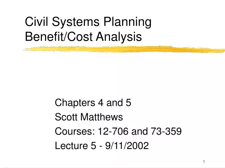
Civil Systems Planning Benefit/Cost Analysis. Chapters 4 and 5 Scott Matthews Courses: 12-706 and 73-359 Lecture 5 - 9/11/2002. Going Over HW #1. Mean = xx (out of 35, xx%) St. dev = xx Min = xx, Max = xx Generally no major problems. Externalities.

E N D
Civil Systems PlanningBenefit/Cost Analysis Chapters 4 and 5 Scott Matthews Courses: 12-706 and 73-359 Lecture 5 - 9/11/2002
Going Over HW #1 • Mean = xx (out of 35, xx%) • St. dev = xx • Min = xx, Max = xx • Generally no major problems 12-706 and 73-359
Externalities • Recall that external effects happen to third parties (non-consumers, producers) • Cause distortions in the market • Are by-products with no markets • Since number of externalities is large, CBA can/should be used before government intervenes to correct 12-706 and 73-359
Pollution (Air or Water) Typical supply functions (MC) only Describe private, not social costs. We assume parallel cost curves P S#:marginal Social costs S*: marginal Private costs P# P* What do these curves, Equilibrium points tell us? D Q Q# Q* 12-706 and 73-359
Pollution (Air or Water) Relatively too much gets produced, At too low of a cost - how to Reduce externality effects? P S#:marginal Social costs S*: marginal Private costs P# P* D Q Q# Q* 12-706 and 73-359
Pollution (Air or Water) Government can charge a tax ‘t’ on Each unit, where t = distance between The two supply curves - What is NSB? P S#:marginal Social costs S*: marginal Private costs P# t P* D Q Q# Q* 12-706 and 73-359
Pollution (Air or Water) CS = (loss) A+B PS=(loss) E+F P S#:marginal Social costs S*: marginal Private costs P# t A B P* F E P# - t D Q Q# Q* 12-706 and 73-359
Pollution (Air or Water) Third parties: (gain) B+C+F (avoided quantity between S curves) Govt revenue: A+E Total: gain of C P S#:marginal Social costs S*: marginal Private costs P# t C A B C is reduced DWL of pollution eliminated by tax P* F E P# - t D Q Q# Q* 12-706 and 73-359
Distorted Market - Vouchers • Example: rodent control vouchers • Give residents vouchers worth $v of cost • Producers subtract $v gov’t pays them • Likely have spillover effects • Neighbors receive benefits since less rodents nearby means less for them too • Thus ‘social demand’ for rodent control is higher than ‘market demand’ 12-706 and 73-359
Distortion : p0,q0 too low What is NSB? What are CS, PS? S P S-v P0 P1 DS: represents WTP For vouchers by all people DM Q Q0 Q1 12-706 and 73-359
Social Surplus - locals What about other people in society, i.e. nearby neighbors? P P S S-v P1+v C A P0 B E P1 DS Because of vouchers, Residents buy Q1 DM Q Q0 Q1 12-706 and 73-359
Nearby Residents Added benefits are area between demand above consumption increase What is cost voucher program? P P S S-v F P1+v C A G P0 B E P1 DS DM Q Q0 Q1 12-706 and 73-359
Voucher Market Benefits • Gain (CS) from target pop: B+E • Gain (CS) in nearby: C+G+F • Producers (PS): A+C • Program cost (vouchers):A+B+C+G+E ---- • Net: C+F 12-706 and 73-359
Opportunity Cost: Land Government decides to buy Q acres of land, pays P per acre What is total cost of project? Price S b P D Q 12-706 and 73-359
Opportunity Cost: Land Government pays PbQ0, but society ‘loses’ CS that they Would have had if government had not bought land. This lost CS is the ‘opportunity cost’ of other people using/buying land. Price S b P D 0 Q 12-706 and 73-359
Another Example: Change in Demand for Concrete Project • If Q high enough, has effect: q’ more • Shifts demand - has supply/price effect • Moves from (P0,Q0) to (P1,Q1).. And?? Price D+q’ D S P1 P0 a Q1 Q0 Quantity 12-706 and 73-359
Another Example: Change in Demand • Original buyers: look at D, buy Q2 • Total purchases still increase by q’ • What is net cost/benefit to society? Price D+q’ D S P1 P0 a Q1 Q2 Q0 Quantity 12-706 and 73-359
Another Example: Change in Demand • Original buyers: look at D, buy Q2 • Project spends B+C+E+F+G on q’ units • Project causes change in social surplus! Price D D+q’ S P1 C A F B P0 G E G G Q1 Q2 Q0 Quantity 12-706 and 73-359
Another Example: Change in Demand • Decrease in CS: A+B (negative) • Increase in PS: A+B+C (positive) • Net social benefit of project is B+G+E+F Price D D+q’ S P1 C A F B P0 G E G G Q1 Q2 Q0 Quantity 12-706 and 73-359
Final Thoughts: Change in Demand • Unless rise in prices high, C negligible • So project outlays ~ social cost • Opp. Cost equals direct expenditures adjusted by social surplus changes Price D S D+q’ P1 C A F B P0 G E G G Q1 Q2 Q0 Quantity 12-706 and 73-359
Secondary Markets • When secondary markets affected • Can and should ignore impacts as long as primary effects measured and undistorted secondary market prices unchanged • Measuring both usually leads to double counting (since primary markets tend to show all effects) 12-706 and 73-359
Primary: Fishing Days Government decides to buy Q acres of land, pays P per acre What is total cost of project? Price a MC0 b MC1 P D Q0 Q1 12-706 and 73-359