Download
1 / 11
120 likes | 274 Views
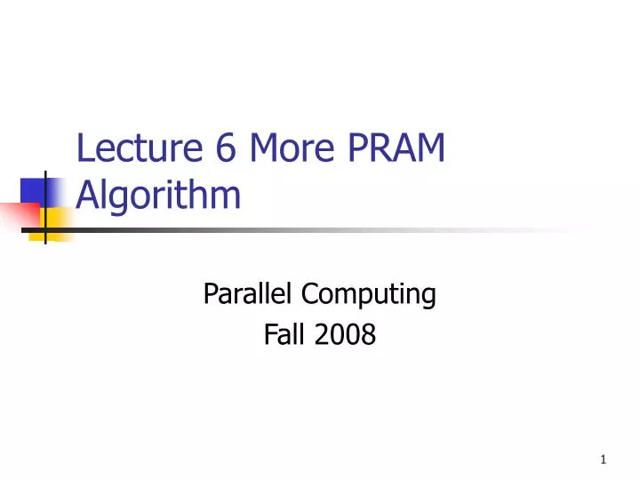
Lecture 6 More PRAM Algorithm. Parallel Computing Fall 2008. Application of Parallel Prefix: Binary Number Addition. Add two n -bit binary numbers in 2 lg n + 1 steps using an n -leaf c.b.t.(complete binary tree) Sequential algorithm requires n steps. Binary addition example:

E N D
Lecture 6 More PRAM Algorithm Parallel Computing Fall 2008
Application ofParallel Prefix: Binary Number Addition • Add two n-bit binary numbers in 2 lg n + 1 steps using an n-leaf c.b.t.(complete binary tree) • Sequential algorithm requires n steps. • Binary addition example: 16 15 14 13 12 11 10 09 08 07 06 05 04 03 02 01 00 a 0 1 0 1 1 1 0 0 1 0 0 1 0 0 1 0 b 0 1 1 0 1 0 0 0 0 1 0 1 1 1 0 0 s g p p g p s s p p s g p p p s s c 0 1 1 1 1 0 0 0 0 0 0 1 0 0 0 0 a +b 1 1 0 0 0 1 0 0 1 1 1 0 1 1 1 0 • (a + b)i = ai ⊕ bi ⊕ ci-1, where ⊕ = XOR. • Signal for each bit: • s: stops a carry bit (0 + 0) • g: generates a carry bit (1 + 1) • p: propagates a carry bit (0 + 1 or 1 + 0).
Application ofParallel Prefix: Binary Number Addition • Problem: In order to compute the k-th carry bit the kth− 1st carry needs to be computed as well. There exists a non-trivial non-obvious parallel solution. • We shall try for each bit position to find the carry bit required for addition so that all bit positions can be added in parallel. We shall show that carry computation takes Θ(lg n) time on a binary tree with a computation that is known to us: parallel prefix. • Observation. The i-th carry bit is one if the leftmost non-p to the right of the i-th bit is a g. • Question. How can we find i-th carry bit?
Application ofParallel Prefix: Binary Number Addition • The previous observation takes the following algorithmic form. Scan for j=i, ... , 0 if p ignore else if g carry=1 exit; else carry=0 exit; • Such a computation requires O(n) time for j = n (n-th bit). Let the i-th bit position symbol (p, s, g) be denoted by xi. Then c0 = x0 = s c1 = x0 ⊗ x1 c2 = x0 ⊗ x1 ⊗ x2 c16 = x0 ⊗ . . . ⊗ x16, where
Application ofParallel Prefix: Binary Number Addition • Algorithm for parallel addition: Step 1. Compute symbol ({s, p, g}) for i bit in parallel for all i. Step 2. Perform a parallel prefix computation on the n symbols plus 0-th symbol s in parallel where operator is defined as in previous table. Step 3. Combine (exclusive OR) the carry bit from bit position i−1 (interpret g as an 1 and an s as a 0) with the exclusive OR of bits in position i to find the i-th bit of the sum. • Steps 1 and 3 require constant time. Step 2, on a complete binary tree on n leaves would require 2 lg n steps. • Totally,T = 1 + 1 + 2lgn. P = 2n −1 = O(n).
Parallel Prefix : Segmented Parallel Prefix (will not be covered) • A segmented prefix (scan) computation consists of a sequence of disjoint prefix computations. Let the xij below take values from a set X and let ⊕ be an associative operator defined on the elements of set X. Then the segmented prefix computation for x11x12. . .x1k1| x21x22. . .x2k2| . . . | xm1xm2. . .xmkm | requires the computation of all pij= xi1⊕ xi2⊕ . . . ⊕ xij ∀ 1 ≤ i ≤ m, 1 ≤ j ≤ ki
Parallel Prefix : Segmented Parallel Prefix (will not be covered) • In brief the segment separator | terminates one prefix operation and starts another one. • One way to deal with a segmented prefix computation in parallel is to extend (X,⊕) into (X,⊗) so that X = X ∪ {|} ∪ {|x : x ∈ X} i.e. X has more than twice the elements of X: it has all the elements of X, the segment separator | and a new element |x which consists of the segment separator and x. The new operator ⊗ is associative if we define it as follows. • Now, if the length of the segmented prefix formula is n we can assign n processors to solve the problem with parallel prefix in asymptotically the same time. Note that an element in X requires for its representation no more than 2 extra bits of the storage size of an element of X. If an ⊕ computation takes O(1) time so does an ⊗ computation. | ⊗ |=| , | ⊗x =|x, | ⊗ |x =|x, x⊗ |=|, |x⊗ |=|, x⊗ y = x ⊕ y |x ⊗ y =|(x ⊕ y) x⊗ |y =|y |x⊗ |y =|y
Parallel Prefix : Segmented Parallel Prefix – Example and Refinements (will not be covered) Example {2, 3} {1, 7, 2} {1, 3, 6}. Create 2 3 |1 7 2|1 3 6. And result is: 2 5|1 8 10|1 4 10. We can refine the previous algorithm as follows.
Problem. Let X1 . . .,XN be n keys. Find X = max{X1,X2, . . .,XN}. The sequential problem accepts a P = 1, T = O(N),W = O(N) direct solution. An EREW PRAM algorithm solution for this problem works the same way as the PARALLEL SUM algorithm and its performance is P = O(N), T = O(lgN),W = O(N lgN),W2 = O(N) along with the improvements in P and W mentioned for the PARALLEL SUM algorithm. In the remainder we will investigate a CRCW PRAM algorithm. Let binary value Xi reside in the local memory of processor i. The CRCW PRAM algorithm MAX1 to be presented has performance T = O(1), P = O(N2), and work W2 = W = O(N2). The second algorithm to be presented in the following pages utilizes what is called a doubly-logarithmic depth tree and achieves T = O(lglgN), P = O(N) and W = W2 = O(N lglgN). The third algorithm is a combination of the EREW PRAM algorithm and the CRCW doubly-logarithmic depth tree-based algorithm and requires T = O(lglgN), P = O(N) and W2 = O(N). PRAM Algorithms:Maximum finding
Maximum Finding: Algorithm MAX1 begin Max1 (X1. . .XN) 1. in proc (i, j) if Xi ≥ Xjthen xij = 1; 2. else xij= 0; 3. Yi= xi1∧ . . . ∧ xin; 4. Processor i reads Yi; 5. if Yi= 1 processor i writes i into cell 0. end Max1 • In the algorithm, we rename processors so that pair (i, j) could refer to processor j × n + i. Variable Yiis equal to 1 if and only if Xiis the maximum. • The CRCW PRAM algorithm MAX1 has performance T = O(1), P = O(N2), and work W2 = W = O(N2).
End Thank you!