Download

1 / 23
250 likes | 266 Views
PRAM Algorithms. Parallel Random Access Machine (PRAM). PRAM instructions execute in 3- phase cycles Read (if any) from a shared memory cell Local computation (if any) Write (if any) to a shared memory cell Processors execute these 3-phase PRAM instructions synchronously.

E N D
Parallel Random Access Machine (PRAM) • PRAM instructions execute in 3- • phase cycles • Read (if any) from a shared memory cell • Local computation (if any) • Write (if any) to a shared memory cell • Processors execute these 3-phase PRAM instructions synchronously • Collection of numbered processors • Access shared memory • Each processor could have local memory (registers) • Each processor can access any shared memory cell in unit time • Input stored in shared memory cells, output also needs to be stored in shared memory
Four Subclasses of PRAM • Four variations: • EREW: Access to a memory location is exclusive. No concurrent read or write operations are allowed. Weakest PRAM model • CREW: Multiple read accesses to a memory location are allowed. Multiple write accesses to a memory location are serialized. • ERCW: Multiple write accesses to a memory location are allowed. Multiple read accesses to a memory location are serialized. Can simulate an EREW PRAM • CRCW: Allows multiple read and write accesses to a common memory location; Most powerful PRAM model; Can simulate both EREW PRAM and CREW PRAM
Concurrent Write Access • arbitraryPRAM: if multiple processors write into a single shared memory cell, then an arbitrary processor succeeds in writing into this cell. • commonPRAM: processors must write the same value into the shared memory cell. • priorityPRAM: the processor with the highest priority (smallest or largest indexed processor) succeeds in writing. • combiningPRAM: if more than one processors write into the same memory cell, the result written into it depends on the combining operator. If it is the sum operator, the sum of the values is written, if it is the maximum operator the maximum is written. Note: An algorithm designed for the common PRAM can be executed on a priority or arbitrary PRAM and exhibit similar complexity. The same holds for an arbitrary PRAM algorithm when run on a priority PRAM.
A Basic PRAM Algorithm • n processors and 2n inputs, find the maximum • PRAM model: EREW • Construct a tournament where values are compared Processor k is active in step j if (k % 2j) == 0 At each step: Compare two inputs, Take max of inputs, Write result into shared memory • Notes: Need to know who is the “parent” and whether you are left or right child; Write to appropriate input field
Finding Maximum: CRCW Algorithm • Find the maximum of n elements A[0, n-1]. • With n2 processors, each processor (i,j) compare A[i] and A[j], for 0<=i, j <=n-1. n=length[A] for i =0 to n-1, in parallel m[i] =true for i =0 to n-1 and j =0 to n-1, in parallel if A[i] < A[j] m[i] =false for i =0 to n-1, in parallel if m[i] =true max = A[i] return max • The running time: O(1). Note: there may be multiple maximum values, so their processors will write to max concurrently.
PRAM Algorithm: Broadcasting • A message (say, a word) is stored in cell 0 of the shared memory. We would like this message to be read by all n processors of a PRAM. • On a CREW PRAM this requires one parallel step (processor i concurrently reads cell 0). • On an EREW PRAM broadcasting can be performed in O(log n) steps. The structure of the algorithm is the reverse of parallel sum. In log n steps the message is broadcast as follows. In step i each processor with index j less than 2ireads the contents of cell j and copies it into cell j + 2i. After log n steps each processor i reads the message by reading the contents of cell i. • A CREW PRAM algorithm that solves the broadcasting problem has performance P = O(n), T = O(1). • The EREW PRAM algorithm that solves the broadcasting problem has performance P = O(n), T = O(log n).
Broadcasting begin Broadcast (M) 1. i = 0 ; j = pid(); C[0]=M; 2. while (2i < P) 3. if (j < 2i) 5. C[j + 2i] = C[j]; 6. i = i + 1; 6. end 7. Processor j reads M from C[j]. end Broadcast
Parallel Prefix • Definition: Given a set of n values x0, x1, . . . , xn−1 and an associative operator, say +, the parallel prefix problem is to compute the following n results/“sums”. 0: x0, 1: x0 + x1, 2: x0 + x1 + x2, . . . n − 1: x0 + x1 + . . . + xn−1. • Parallel prefix is also called prefix sums or scan. It has many uses in parallel computing such as in load-balancing the work assigned to processors and compacting data structures such as arrays. • We shall prove that computing ALL THE SUMS is no more difficult that computing the single sum x0 + . . .xn−1.
Parallel Prefix Algorithm • An algorithm for parallel prefix on an EREW PRAM would require log n phases. In phase i, processor j reads the contents of cells j and j − 2i(if it exists) combines them and stores the result in cell j. • The EREW PRAM algorithm that solves the parallel prefix problem has performance P = O(n), T = O(log n).
Parallel Prefix Example For visualization purposes, the second step is written in two different lines. When we write x1 + . . . + x5 we mean x1 + x2 + x3 + x4 + x5. x1 x2 x3 x4 x5 x6 x7 x8 1. x1+x2 x2+x3 x3+x4 x4+x5 x5+x6 x6+x7 x7+x8 2. x1+(x2+x3) (x2+x3)+(x4+x5) (x4+x5)+(x6+x7) 2. (x1+x2)+(x3+x4) (x3+x4)+(x5+x6) (x5+x6+x7+x8) 3. x1+...+x5 x1+...+x7 3. x1+...+x6 x1+...+x8 Finally F. x1 x1+x2 x1+...+x3 x1+...+x4 x1+...+x5 x1+...+x6 x1+...+x7 x1+...+x8
Parallel Prefix Example For visualization purposes, the second step is written in two different lines. When we write [1 : 5] we mean x1 +x2 + x3 + x4 + x5. We write below [1:2] to denote x1+x2 [i:j] to denote xi + ... + x5 [i:i] is xi NOT xi+xi! [1:2][3:4]=[1:2]+[3:4]= (x1+x2) + (x3+x4) = x1+x2+x3+x4 A * indicates value above remains the same in subsequent steps 0 x1 x2 x3 x4 x5 x6 x7 x8 0 [1:1] [2:2] [3:3] [4:4] [5:5] [6:6] [7:7] [8:8] 1 * [1:1][2:2] [2:2][3:3] [3:3][4:4] [4:4][5:5] [5:5][6:6] [6:6][7:7] [7:7][8:8] 1. * [1:2] [2:3] [3:4] [4:5] [5:6] [6:7] [7:8] 2. * * [1:1][2:3] [1:2][3:4] [2:3][4:5] [3:4][5:6] [4:5][6:7] [5:6][7:8] 2. * * [1:3] [1:4] [2:5] [3:6] [4:7] [5:8] 3. * * * * [1:1][2:5] [1:2][3:6] [1:3][4:7] [1:4][5:8] 3. * * * * [1:5] [1:6] [1:7] [1:8] [1:1] [1:2] [1:3] [1:4] [1:5] [1:6] [1:7] [1:8] x1 x1+x2 x1+x2+x3 x1+...+x4 x1+...+x5 x1+...+x6 x1+...+x7 x1+...+x8
Parallel Prefix Algorithm // We write below[1:2] to denote X[1]+X[2] // [i:j] to denote X[i]+X[i+1]+...+X[j] // [i:i] is X[i] NOT X[i]+X[i] // [1:2][3:4]=[1:2]+[3:4]= (X[1]+X[2])+(X[3]+X[4])=X[1]+X[2]+X[3]+X[4] // Input : M[j]= X[j]=[j:j] for j=1,...,n. // Output: M[j]= X[1]+...+X[j] = [1:j] for j=1,...,n. ParallelPrefix(n) 1. i=1; // At this step M[j]= [j:j]=[j+1-2**(i-1):j] 2. while (i < n ) { 3. j=pid(); 4. if (j-2**(i-1) >0 ) { 5. a=M[j]; // Before this stepM[j] = [j+1-2**(i-1):j] 6. b=M[j-2**(i-1)]; // Before this stepM[j-2**(i-1)]= [j-2**(i-1)+1-2**(i-1):j-2**(i-1)] 7. M[j]=a+b; // After this step M[j]= M[j]+M[j-2**(i-1)]=[j-2**(i-1)+1-2**(i-1):j-2**(i-1)] // [j+1-2**(i-1):j] = [j-2**(i-1)+1-2**(i-1):j]=[j+1-2**i:j] 8. } 9. i=i*2; } At step 5, memory location j − 2i−1 is read provided that j − 2i−1≥ 1. This is true for all times i ≤ tj = log(j − 1) + 1. For i > tj the test of line 4 fails and lines 5-8 are not executed.
Logical AND Operation Problem. Let X1. . .,Xnbe binary/boolean values. Find X = X1∧ X2∧ . . . ∧ Xn. • The sequential problem : T = O(n). • An EREW PRAM algorithm solution for this problem works the same way as the PARALLEL SUM algorithm and its performance is P = O(n), T = O(log n). • A CRCW PRAM algorithm: Let binary value Xireside in the shared memory location i. We can find X = X1∧ X2 ∧ . . . ∧ Xnin constant time on a CRCW PRAM. Processor 1 first writes an 1 in shared memory cell 0. If Xi= 0, processor i writes a 0 in memory cell 0. The result X is then stored in this memory cell. • The result stored in cell 0 is 1 (TRUE) unless a processor writes a 0 in cell 0; then one of the Xiis 0 (FALSE) andthe result X should be FALSE,
Logical AND Operation begin Logical AND (X1 . . .Xn) 1. Proc 1 writ1es in cell 0. 2. if Xi= 0 processor i writes 0 into cell 0. end Logical AND Exercise: Give an O(1) CRCW algorithm for Logical OR
Matrix Multiplication Matrix Multiplication • A simple algorithm for multiplying two n × n matrices on a CREW PRAM with time complexity T = O(log n) using P = n3 processors. For convenience, processors are indexed as triples (i, j, k), where i, j, k = 1, . . . , n. In the first step processor (i, j, k) concurrently reads aijand bjkand performs the multiplication aijbjk. In the following steps, for all i, k the results (i, ∗, k) are combined, using the parallel sum algorithm to form cik= j aijbjk. After logn steps, the result cikis thus computed. • The same algorithm also works on the EREW PRAM with the same time and processor complexity. The first step of the CREW algorithm need to be changed only. We avoid concurrency by broadcasting element aijto processors (i, j, ∗) using the broadcasting algorithm of the EREW PRAM in O(log n) steps. Similarly, bjkis broadcast to processors (∗, j, k). • The above algorithm also shows how an n-processor EREW PRAM can simulate an n-processor CREW PRAM with an O(log n) slowdown.
Matrix Multiplication CREW EREW 1. aij to all (i,j,*) procs O(1) O(logn) bjk to all (*,j,k) procs O(1) O(logn) 2. aij*bjk at (i,j,k) proc O(1) O(1) 3. parallel sumj aij *bjk (i,*,k) procs O(logn) O(logn) n procs participate 4. cik = sumj aij*bjkO(1) O(1) T=O(logn),P=O(n3 )
Parallel Sum(Compute x0 + x1 + . . . + xn−1) Algorithm Parallel Sum. M[0] M[1] M[2] M[3] M[4] M[5] M[6] M[7] x0 x1 x2 x3 x4 x5 x6 x7 t=0 x0+x1 x2+x3 x4+x5 x6+x7 t=1 x0+...+x3 x4+...+x7 t=2 x0+...+x7 t=3 • This EREW PRAM algorithm consists of log n steps. In step i, if j can be exactly divisible by 2i, processor j reads shared-memory cells j and j + 2i-1 combines (sums) these values and stores the result into memory cell j. After logn steps the sum resides in cell 0. Algorithm Parallel Sum has T = O(log n), P = n. Processing node used: P0, P2, P4, P6 t=1 P0, P4 t=2 P0 t=3
Parallel Sum(Compute x0 + x1 + . . . + xn−1) // pid() returns the id of the processor issuing the call. begin Parallel Sum (n) 1. i = 1 ; j = pid(); 2. while (j mod2i == 0) 3. a = C[j]; 4. b = C[j + 2i-1]; 5. C[j] = a + b; 6. i = i + 1; 7. end end Parallel Sum
Parallel Sum(Compute x0 + x1 + . . . + xn−1) • Sequential algorithm: n − 1 additions. • A PRAM implementation: value xiis initially stored in shared memory cell i. The sum x0 + x1 + . . . + xn−1 is to be computed in T = logn parallel steps. Without loss of generality, let n be a power of two. • If a combining CRCW PRAM with arbitration rule sum is used to solve this problem, the resulting algorithm is quite simple. In the first step processor i reads memory cell i storing xi. In the following step processor i writes the read value into an agreed cell say 0. The time is T = O(1), and processor utilization is P = O(n). • A more interesting algorithm is the one presented below for the EREW PRAM. The algorithm consists of log n steps. In step i, processor j < n / 2ireads shared-memory cells 2j and 2j +1 combines (sums) these values and stores the result into memory cell j. After logn steps the sum resides in cell 0. Algorithm Parallel Sum has T = O(log n), P = n.
Parallel Sum(Compute x0 + x1 + . . . + xn−1) // pid() returns the id of the processor issuing the call. begin Parallel Sum (n) 1. i = 1 ; j = pid(); 2. while (j < n / 2i) 3. a = C[2j]; 4. b = C[2j + 1]; 5. C[j] = a + b; 6. i = i + 1; 7. end end Parallel Sum
Parallel Sum Example M[0] M[1] M[2] M[3] M[4] M[5] M[6] M[7] x0 x1 x2 x3 x4 x5 x6 x7 t=0 x0+x1 x2+x3 x4+x5 x6+x7 t=1 x0+...+x3 x4+...+x7 t=2 x0+...+x7t=3
Parallel Sum • Can be easily extended to the case where n is not a power of two. • The first instance of a sequential problem that has a trivial sequential but more complex parallel solution. • Any associative operator can be used. As associative operator ⊗ is one such that (a ⊗ b) ⊗ c = a ⊗(b ⊗ c)