Download
1 / 35
350 likes | 480 Views
An OSSE-based evaluation of 4D- Ensemble-Var (and hybrid variants) for the NCEP GFS. 1 NOAA/NWS/NCEP/EMC 2 Univ. of Maryland-College Park, Dept. of Atmos. & Oceanic Science. Daryl Kleist 1,2 and Kayo Ide 2. w ith acknowledgements to Dave Parrish, Jeff Whitaker, John Derber , Russ Treadon.

E N D
An OSSE-based evaluation of 4D-Ensemble-Var (and hybrid variants) for the NCEP GFS 1NOAA/NWS/NCEP/EMC 2Univ. of Maryland-College Park, Dept. of Atmos. & Oceanic Science Daryl Kleist1,2 and Kayo Ide2 with acknowledgements to Dave Parrish, Jeff Whitaker, John Derber, Russ Treadon CMOS 2012 Congress AMS 21st NWP and 25th WAF Conferences Montréal, Québec, Canada -- 29 May to 01 June 2012
Outline • Introduction • Background on hybrid data assimilation • Hybrid 3DVAR/EnKF experiments with GFS using an OSSE • 4D-Ensemble-Var • Evaluation using OSSE framework • Hybridization with time invariant static B
IncrementalVariational Data Assimilation J : Penalty (Fit to background + Fit to observations) x’ : Analysis increment (xa – xb) ; where xb is a background Bf : (Fixed) Background error covariance H : Observations (forward) operator R : Observation error covariance (Instrument + representativeness) , where yo are the observations Cost function (J) is minimized to find solution, x’ [xa=xb+x’] 3 B is typically static and estimated a-priori/offline
Motivation from [Ensemble]Kalman Filter • Problem: dimensions of AKF and BKF are huge, making this practically impossible for large systems (GFS for example) • Solution: sample and update using an ensemble instead of evolving AKF and BKF explicitly Forecast Step: Ensemble Perturbations Analysis Step: N is ensemble size
Hybrid Variational-Ensemble • Incorporate ensemble perturbations directly into variational cost function through extended control variable • Lorenc (2003), Buehner (2005), Wang et. al. (2007), etc. bf & be: weighting coefficients for fixed and ensemble covariance respectively xt’: (total increment) sum of increment from fixed/static B (xf’) and ensemble B ak: extended control variable; :ensemble perturbations - analogous to the weights in the LETKF formulation L: correlation matrix [effectively the localization of ensemble perturbations]
Single Temperature Observation 3DVAR bf-1=0.0 bf-1=0.5
Outline • Introduction • Background on hybrid data assimilation • Hybrid 3DVAR/EnKF Experiments with GFS using an OSSE • 4D-Ensemble-Var • Evaluation using OSSE framework • Hybridization with time invariant static B
Observing System SimulationExperiments (OSSE) • Typically used to evaluate impact of future observing systems • Doppler-winds from spaced-based lidar, for example • Useful for evaluating present/proposed data assimilation techniques since ‘truth’ is known • Series of experiments are carried out to test hybrid variants • Joint OSSE • International, collaborative effort between ECMWF, NASA/GMAO, NOAA (NCEP/EMC, NESDIS, JCSDA), NOAA/ESRL, others • ECMWF-generated nature run (c31r1) • T511L91, 13 month free run, prescribed SST, snow, ice
Synthetic Observations • Observations from (operational) 2005/2006 observing system developed • NCEP: ‘conventional’, sbuv ozone retrievals, GOES sounder radiances • NASA/GMAO: all other radiances (AMSUA/B, HIRS, AIRS, MSU) • Older version of the CRTM • Simulated observation errors developed by Ron Errico (GMAO/UMBC) • Horizontally correlated errors for radiances • Vertically correlated errors for conventional soundings • Synthetic observations used in this study were calibrated by Nikki Prive (GMAO) • Attempt to match impact of various observation types with results from data denial experiments 9 *Thanks to Ron and Nikki for all of their help in getting/using the calibrated synthetic observations.
Availability of SimulatedObservations [00z 24 July] SURFACE/SHIP/BUOY SONDES AMSUA/MSU AIRS/HIRS AMVS AIRCRAFT PIBAL/VADWND/PROFLR SSMI SFC WIND SPD AMSUB GOES SOUNDER
3D Experimental Design • Model • NCEP Global Forecast System (GFS) model (T382L64; post May 2011 version – v9.0.1) • Test Period • 01 July 2005-31 August 2005 (3 weeks ignored for spin-up) • Observations • Calibrated synthetic observations from 2005 observing system (courtesy Ron Errico/Nikki Privi) • 3DVAR • Control experiment with standard 3DVAR configuration (increment comparison to real system) • 3DHYB • Ensemble (T190L64) • 80 ensemble members, EnSRF update, GSI for observation operators • Additive and multiplicative inflation • Dual-resolution, 2-way coupled • High resolution control/deterministic component • Ensemble is recentered every cycle about hybrid analysis • Discard ensemble mean analysis • Parameter settings • bf-1=0.25, be-1=0.75 [25% static B, 75% ensemble] • Level-dependent localization
3DVAR Time MeanIncrement Comparison U T Ps (BACK) OSSE REAL
3DHYB Details • Full B preconditioned double conjugate gradient minimization • Spectral filter for horizontal part of L • Eventually replace with (anisotropic) recursive filters • Recursive filter used for vertical • 0.5 scale heights • Same localization used in Hybrid (L) and EnSRF • TLNMC (Kleist et al. 2009) applied to total analysis increment* *TLNMC is also applied to increment in 3DVAR experiment.
Dual-Res Coupled Hybrid Var/EnKF Cycling Generate new ensemble perturbations given the latest set of observations and first-guess ensemble member 1 forecast member 1 analysis T190L64 EnKF member update member 2 forecast member 2 analysis recenter analysis ensemble member 3 analysis member 3 forecast Ensemble contribution to background error covariance Replace the EnKF ensemble mean analysis GSI Hybrid Ens/Var high res forecast high res analysis T382L64 Previous Cycle Current Update Cycle
Time Series of Analysis andBackground Errors • Solid (dashed) show background (analysis) errors • 3DHYB background errors generally smaller than 3DVAR analysis errors (significantly so for zonal wind) • Strong diurnal signal for temperature errors due to availability of rawinsondes 500 hPa U 850 hPa T
3DVAR and 3DHYBAnalysis Errors U T Q 3DVAR 3DHYB 3DHYB-3DVAR
Zonal Wind BackgroundErrors 3DHYB 3DVAR BEN Bf
3D Follow-on Experiments • To further understand some of the degradation, two-additional 3D experiments are designed • 3DENSV • 3DHYB re-run, but with no static B contribution (bf-1=0.0) • Analogous to a dual-resolution 3D-EnKF (but solved variationally) • 3DHYB_RS (Reduced Spread) • Inflation parameters reduced to produce a better match between ensemble spread and actual F06 error
3DENSV Analysis Error U • Same problem areas from 3DHYB (error increase) reappear • Ensemble covariances improve tropics • New problem areas arise (static B really helps, especially with imperfect ensemble) T Q 3DENSV-3DVAR
3DHYB_RS U T New (RS) hybrid experiment almost uniformly better than 3DVAR Inflation still a necessary evil (move to adaptive?) Q 3DHYB_RS-3DVAR
Summary of 3D Experiments • 3DHYB generally better than 3DVAR • Hybrid background errors smaller than 3DVAR analysis errors • Significant improvement in tropics (smaller improvements in extratropics) • Quality of ensemble can have impact on quality of analysis • Need for adaptive inflation • Stochastic physics, localization, ensemble size • Hybrid helps mitigate (some) problems with imperfect ensemble
Outline • Introduction • Background on hybrid data assimilation • Hybrid 3DVAR/EnKF Experiments with GFS using an OSSE • 4D-Ensemble-Var • Evaluation using OSSE framework • Hybridization with time invariant static B
Hybrid ensemble-4DVAR[H-4DVAR_AD] Incremental 4DVAR: bin observations throughout window and solve for increment at beginning of window (x0’). Requires linear (M) and adjoint (MT) models Can be expanded to include hybrid just as in the 3DHYB case With a static and ensemble contribution to the increment at the beginning of the window
4D-Ensemble-Var[4DENSV] As in Buehner et al. (2010), the H-4DVAR_AD cost function can be modified to solve for the ensemble control variable (without static contribution) Where the 4D increment is prescribed exclusively through linear combinations of the 4D ensemble perturbations Here, the control variables (ensemble weights) are assumed to be valid throughout the assimilation window (analogous to the 4D-LETKF without temporal localization). Note that the need for the computationally expensive linear and adjoint models in the minimization is conveniently avoided.
Hybrid 4D-Ensemble-Var[H-4DENSV] The 4DENSV cost function can be easily expanded to include a static contribution Where the 4D increment is prescribed exclusively through linear combinations of the 4D ensemble perturbations plus static contribution Here, the static contribution is considered time-invariant (i.e. from 3DVAR-FGAT). Weighting parameters exist just as in the other hybrid variants.
Single Observation (-3h) Examplefor 4D Variants 4DVAR 4DENSV H-4DVAR_AD bf-1=0.25 H-4DENSV bf-1=0.25
Time Evolution of Increment Solution at beginning of window same to within round-off (because observation is taken at that time, and same weighting parameters used) Evolution of increment qualitatively similar between dynamic and ensemble specification ** Current linear and adjoint models in GSI are computationally unfeasible for use in 4DVAR other than simple single observation testing at low resolution t=-3h t=0h t=+3h H-4DENSV H-4DVAR_AD
4D OSSE Experiments • To investigate the use of 4D ensemble perturbations, two new OSSE based experiments are carried out. • The original (not reduced) set of inflation parameters are used. • Exact configuration as was used in the 3D OSSE experiments, but with 4D features • 4DENSV • No static B contribution (bf-1=0.0) • Analogous to a dual-resolution 4D-EnKF (but solved variationally) • To be compared with 3DENSV • H-4DENSV • 4DENSV + addition of time invariant static contribution (bf-1=0.25) • This is the non-adjoint formulation • To be compared with 4DENSV
Impact on Analysis Errors U T Q H-4DENSV-4DENSV 4DENSV-3DENSV
Dynamic Constraints • One advantage of the variational framework is ease in which one can apply dynamic constraints on the solution • Several constraint options have been developed and explored for use with the 4DENSV algorithm • Tangent linear normal mode constraint • Weak constraint digital filter • Combined normal mode/digital filter
Comparison of 3DHYB andH-4DENSV (with dynamic constraints) U T Something in the 4D experiments is resulting in more moisture in the analysis, triggering more convective precipitation Q 4DHYB-3DHYB
Summary of 4D Experiments • 4DENSV seems to be a cost effective alternative to 4DVAR • Inclusion of time-invariant static B to 4DENSV solution is beneficial for dual-resolution paradigm • Extension to 4D seems to have larger impact in extratropics (whereas the original introduction of the ensemble covariances had largest impact in the tropics) • Moisture constraint and/or observations contributing to increased convection in 4D extensions • Original tuning parameters for inflation were utilized. Follow-on experiments with tuned parameters (reduced inflation) and/or adapative inflation should yield even more impressive results.
Summary and Conclusions • Analysis errors are reduced when using a hybrid algorithm relative to 3DVAR • Inclusion of a static B contribution proved beneficial to 3D and 4D variants when using a dual-resolution configuration • Extension to 4D ensemble has larger impact in extratropics whereas the introduction of the ensemble covariance estimate had largest impact in the tropics • Quality of analyses sensitive to quality of ensemble. Care needs to be taken in specifying certain aspects such as inflation parameters
Future Work • Comparison of 4DENSV variants with 4DVAR in OSSE context • Follow-on OSSE experiments to better understand what is leading to increase in moisture (therefore exciting more convection) in the 4D experiments relative to 3D • Testing of H-4DENSV (with constraint) using real observations. This configuration is what I envision being a prototype for future operational implementation • Temporal (and variable?) localization in hybrid • Hybrid Weighting Variations(b) • Piecewise scale-dependent (already coded, preliminary testing compled) • Fully adaptive (weights as a control variable?) • Hybridization of EnKF update • LETKF instead of EnSRF (?) • Adaptive Inflation • Observation impact estimation within hybrid DA • QOL/RIP within 4DENSV variants
Operational (3D) Hybrid • Implemented into GDAS/GFS at 12z 22 May 2012 1000 mb NH 500 mb SH 3DHYB-3DVAR