Download
1 / 42

E N D
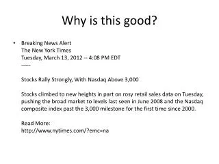
Why is this good? • Breaking News AlertThe New York TimesTuesday, March 13, 2012 -- 4:08 PM EDT-----Stocks Rally Strongly, With Nasdaq Above 3,000Stocks climbed to new heights in part on rosy retail sales data on Tuesday, pushing the broad market to levels last seen in June 2008 and the Nasdaq composite index past the 3,000 milestone for the first time since 2000. Read More:http://www.nytimes.com/?emc=na
AD/AS What causes short run changes in the business cycle?
Aggregate Supply Aggregate Demand
Business cycle Economic activity Time The Model of Aggregate Demand and Aggregate Supply • Economist use the model of aggregate demand and aggregate supply to explain short-run fluctuations in economic activity around its long-run trend. http://www.youtube.com/watch?v=hTWPrWmPJS0
The Model of Aggregate Demand and Aggregate Supply • The aggregate-demand curve shows the quantity of goods and services that households, firms, and the government want to buy at each price level. • The aggregate-supply curve shows the quantity of goods and services that firms choose to produce and sell at each price level. Sum each definition in six words or less!!!
Aggregate supply Equilibrium price level Aggregate demand Equilibrium output Figure 2 Aggregate Demand and Aggregate Supply... Price Level How do we measure price level? PPI CPI Price Deflator Quantity of 0 Output
P P2 1. A decrease Aggregate in the price demand level . . . Y Y2 2. . . . increases the quantity of goods and services demanded. Figure 3 The Aggregate-Demand Curve... Price Level WHY??? Quantity of 0 Output
Why the Aggregate-Demand Curve Is Downward Sloping • The Price Level and Consumption: • The Wealth Effect • The Price Level and Investment: • The Interest Rate Effect • The Price Level and Net Exports: • The Exchange-Rate Effect
Why the Aggregate-Demand Curve Is Downward Sloping • The Price Level and Consumption: • The Wealth Effect • A lower price level raises the real value of money and makes consumers wealthier, which encourages them to spend more. • This increase in consumer spending means larger quantities of goods and services demanded.
Why the Aggregate-Demand Curve Is Downward Sloping • The Price Level and Investment: • The Interest Rate Effect • A lower price level reduces the interest rate and makes borrowing less expensive, which encourages greater spending on investment goods. • This increase in investment spending means a larger quantity of goods and services demanded.
Why the Aggregate-Demand Curve Is Downward Sloping • The Price Level and Net Exports: • The Exchange-Rate Effect • A lower price level in the U.S. causes U.S. interest rates to fall and the real exchange rate to depreciate, which stimulates U.S. net exports. • The increase in net export spending means a larger quantity of goods and services demanded.
Aggregate Demand Aggregate Demand can either increase or decrease depending on which variables shift the aggregate demand curve. An increase in aggregate demand is always a shift to the right A decrease in aggregate demand is always a shift to the left. PL Ad Ad1 Ad1 Q=Real GDP=Y
Variables Affecting the Components
Variables that influence the components- Aggregate Demand C onsumption Relative prices of products/services People’s preferences/tastes Expectations of the future Change in interest rates Change in income
Variables that influence the components- Aggregate Demand I Number of consumers nvestment People’s preferences/tastes Expectations of the future profit Change in Inventories Change in Interest rates Change in income Gross Private Domestic Business Investment
Variables that influence the components- Aggregate Demand G overnment Spending Dum Politicians b
Variables that influence the components- Aggregate Demand (X - M) Relative quality of foreign goods/services Relative price of foreign goods/services Exports Imports International value of the dollar Interest rates
Variables that influence the components- Aggregate Demand S avings Relative prices of products/services People’s preferences/tastes Expectations of the future Change in Interest rates Change in income
Demand Shifts - Summary • Federal government increases personal income tax rates • Federal Reserve implements “tight” monetary policy • News media runs several stories showing economy in positive light • U.S. currency exchange rate depreciates against the Yuan (Chinese currency). • People increase savings rates • Construction of new housing increases
As PL Classical Range http://logic.csc.cuhk.edu.hk/~b024765/ricardo.jpg http://logic.csc.cuhk.edu.hk/~b024765/smith.jpg http://logic.csc.cuhk.edu.hk/~b024765/say.jpg COVER BY JOHN HELD JR. http://www.sntc.org.sz/sdphotos/1880s.html http://www.nytimes.com/learning/general/onthisday/bday/0605.html http://logic.csc.cuhk.edu.hk/~b024765/keynes.jpg Intermediate Range Full Employment Keynesian Range Q = Real GDP = Y
As PL Structural Frictional Cyclical Unemployment Classical Range Intermediate Range Full Employment Keynesian Range Q = Real GDP = Y
THE AGGREGATE-SUPPLY CURVE • In the long run, the aggregate-supply curve is vertical because the price level does not affect long run determinants of real GDP. • In the short run, the aggregate-supply curve is upward sloping.
THE AGGREGATE-SUPPLY CURVE • In the long run, an economy’s production of goods and services depends on its supplies of labor, capital, and natural resources and on the available technology used to turn these factors of production into goods and services. • The price level does not affect these variables in the long run. • The long-run aggregate supply represents the classical dichotomy and money neutrality.
Long-run aggregate supply P P2 2. . . . does not affect 1. A change the quantity of goods in the price and services supplied level . . . in the long run. Figure 4 The Long-Run Aggregate-Supply Curve Price Level Quantity of 0 Natural rate Output of output
Why the Long-Run Aggregate-Supply Curve Might Shift • Shifts might arise from changes in: • Labor • Capital • Natural Resources • Technological Knowledge
2. . . . and growth in the Long-run money supply shifts aggregate aggregate demand . . . supply, LRAS LRAS LRAS 1980 1990 2000 1. In the long run, technological progress shifts long-run aggregate P 2000 supply . . . 4. . . . and ongoing inflation. P 1990 Aggregate Demand, AD 2000 P 1980 AD 1990 AD 1980 Y Y Y 1980 1990 2000 3. . . . leading to growth in output . . . Figure 5 Long-Run Growth and Inflation Price Level Quantity of 0 Output
Why the Aggregate-Supply Curve Slopes Upward in the Short Run • In the short run, an increase in the overall level of prices in the economy tends to raise the quantity of goods and services supplied. • A decrease in the level of prices tends to reduce the quantity of goods and services supplied. • As a result, the short-run aggregate-supply curve is upward sloping.
Short-run aggregate supply P P2 2. . . . reduces the quantity 1. A decrease of goods and services in the price supplied in the short run. level . . . Y2 Y Figure 6 The Short-Run Aggregate-Supply Curve Price Level Quantity of 0 Output
Why the Aggregate-Supply Curve Slopes Upward in the Short Run • Three Theories: • The Sticky-Wage Theory • The Sticky-Price Theory • The Misperceptions Theory
Why the Aggregate-Supply Curve Slopes Upward in the Short Run • The Sticky-Wage Theory • Nominal wages are slow to adjust to changing economic conditions, or are “sticky” in the short run
Why the Aggregate-Supply Curve Slopes Upward in the Short Run • The Sticky-Price Theory • An unexpected fall in the price level leaves some firms with higher-than-desired prices. For a variety of reasons, they may not want to or be able to change prices immediately.
Why the Aggregate-Supply Curve Slopes Upward in the Short Run • The Misperceptions Theory • Changes in the overall price level temporarily mislead suppliers about what is happening in the markets in which they sell their output. • A lower price level causes misperceptions about relative prices. • These misperceptions induce suppliers to decrease the quantity of goods and services supplied.
Why the Short-Run Aggregate-Supply Curve Might Shift • Shifts might arise from changes in: • Expected Price Level. • Labor. • Capital. • Natural Resources. • Technology. COSTS!!!!
Long-run aggregate Short-run supply aggregate supply A Equilibrium price Aggregate demand Natural rate of output Figure 7 The Long-Run Equilibrium Price Level Quantity of 0 Output
TWO CAUSES OF ECONOMIC FLUCTUATIONS • Four steps in the process of analyzing economic fluctuations: • Determine whether the event affects aggregate supply or aggregate demand. • Decide which direction the curve shifts. • Use a diagram to compare the initial and the new equilibrium. • Keep track of the short and long run equilibrium, and the transition between them.
2. . . . causes output to fall in the short run . . . Short-run aggregate supply, AS AS2 3. . . . but over time, the short-run A aggregate-supply P curve shifts . . . B P2 1. A decrease in aggregate demand . . . P3 C Aggregate demand, AD AD2 Y2 Y 4. . . . and output returns to its natural rate. Figure 8 A Contraction in Aggregate Demand Price Level Long-run aggregate supply Quantity of 0 Output
1. An adverse shift in the short- run aggregate-supply curve . . . Short-run AS2 aggregate supply, AS B P2 A P 3. . . . and the price level to rise. Aggregate demand Y2 Y 2. . . . causes output to fall . . . Figure 10 An Adverse Shift in Aggregate Supply Price Level Long-run aggregate supply Quantity of 0 Output
The Effects of a Shift in Aggregate Supply • Adverse shifts in aggregate supply cause stagflation—a period of recession and inflation. • Output falls and prices rise. • Policymakers who can influence aggregate demand cannot offset both of these adverse effects simultaneously.
The Effects of a Shift in Aggregate Supply • Policy Responses to Recession • Policymakers may respond to a recession in one of the following ways: • Do nothing and wait for prices and wages to adjust. • Take action to increase aggregate demand by using monetary and fiscal policy.
1. When short-run aggregate supply falls . . . Short-run AS2 aggregate supply, AS P3 C 2. . . . policymakers can accommodate the shift P2 by expanding aggregate A 3. . . . which demand . . . P causes the price level AD2 to rise 4. . . . but keeps output further . . . at its natural rate. Figure 11 Accommodating an Adverse Shift in Aggregate Supply Price Level Long-run aggregate supply Aggregate demand, AD Quantity of 0 Natural rate Output of output