Download
1 / 60
600 likes | 715 Views
Ch.3. AGN. the term Active Galactic Nuclei (AGN) refers to the existence of energetic phenomena in the central regions of galaxies, phenomena which cannot be attributed clearly and directly to stars. 2 main classes were initially found:

E N D
AGN the term Active Galactic Nuclei (AGN) refers to the existence of energetic phenomena in the central regions of galaxies, phenomena which cannot be attributed clearly and directly to stars 2 main classes were initially found: 1) Seyfert galaxies luminosity ~1044 erg/s (~galaxy) 2) quasar luminosity > 1044 erg/s even 1046-1047 erg/s same phenomenon, but initially the two classes were selected with different criteria 1) galaxies with bright nucleus 2) high luminosity objects, apparently not in galaxies rare in the nearby Universe, thus hardly referable to galaxies
Seyfert galaxies 1908, Fath, Lick Observatory: first optical spectrum of a Seyfert galaxy, strong emission lines in NGC 1068 1917, Slipher, Lowell Observatory: confirmation, line width several hundreds km/s 1943, Seyfert: selects a sample of galaxies with high central surface brightness (nucleus with stellar appearence) NGC 1068, NGC 1275, NGC 3516, NGC 4051, NGC 4151, NGC 7469 spectra contain high excitation emission lines important characteristics of spectra: 1) broad lines up to ~8500 km/s FWZI (Full Width at Zero Intensity) 2) Hydrogen lines sometimes larger than other lines 1955, NGC 1068 and NGC 1275 discovered radiosources 1959 Woltjer, first trial to understand physics of Seyfert galaxies: 1) non resolved nuclei, r < 100 pc 2) duration of emission > 108 yr, in fact Seyferts ~ 1/100 galaxies 3) if matter in nucleus is gravitationally bound, then Virial Theorem:
radio surveys quasars originally discovered as radiosources, identified with optical objects with stellar appearence 3C and 3CR third Cambridge catalog (Edge et al 1959) 158 MHz and revision (Bennett 1961) 178 MHz flux limit 9 Jy [ 1 Jy (Jansky)=10-26 W/m2/Hz=10-23 erg/s/cm2/Hz ] declination > -22o (3C), > -5o (3CR) but sample limited by confusion limit: many faint sources close in the sky, within ~1 degree resolution 3C: 471 sources, 3CR: 328 sources, numbered sequentially in RA, e.g. 3C273, 3C390.3 (decimal digit: sources added in 3CR) 3C390.3 VLA 1565 MHz Wilkinson et al. (1991) 3C273 Merlin 408 MHz 3C273 optical image
radio surveys PKS survey of the southern sky (<+25o) performed at Parkes, Australia (Ekers 1969) 408 MHz (Slim=4 Jy), 1410 MHz (1 Jy), 2650 MHz (0.3 Jy) sources named by position (1950 coordinates), e.g. 3C273 = PKS 1226+023 : 12h 26m +02o.3 4C fourth Cambridge catalog (Pilkington & Scott 1965, Gower et al. 1967) 178 MHz, 2 Jy named by declination and sequential number, e.g. 3C273=4C 02.32 (source no. 32 between 02 and 03 declination degrees) AO Arecibo occultation survey (Hazard et al. 1967) extremely accurate positions obtained through lunar occultation named by position OHIO (Ehman et al 1979), 1415 MHz names Ox yyy, where x progressive letter indicating RA (except A, O), and yyy sequential number e.g. 3C273=ON 044 [N: between 12h and 13h]
radio surveys most radiosources were identified with galaxies in some cases instead, position coincided with starlike objects, e.g. on Palomar Sky Survey plates first powerful radiosource identified with a pointlike object was 3C48, Matthews & Sandage (1963): optical counterpart was a 16 mag star 3C48 Merlin 1666MHz however, the spectrum was anomalous, with very broad emission lines, and at apparently unknown wavelengths z=0.367
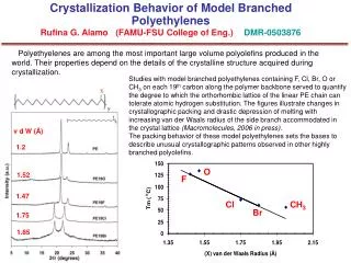
3C 273 6566x1.158=7603 z=0.158 4861x1.158=5629
Maarten Schmidt 3C273. Maarten Schmidt understood (1963) that emission lines were related to Balmer Hydrogen series, and to MgII transition (2798Å), at the quite large redshift z=0.158 => large distance: distance modulus => high luminosity ~100x Milky Way (cf MB ~ -21)
quasars Schmidt, quasar general properties: • objects with stellar appearence identified with radiosources • variable continuum flux • large UV flux • broad emission lines • high redshifts however, not all the objects now called AGNs possess all these properties and other properties have later resulted important: e.g. one property which seems to be shared by all AGNs is a high X-ray luminosity (Elvis et al 1978) in modern terms, one quasar characteristic is a very extended SED (spectral energy distribution) AGNs cannot be described in terms of black-body emission, non-thermal processes are needed, e.g. synchrotron stars (~black body)
SED typically, for a given frequency interval, it is used a power-law (but sometimes the spectral index is defined with implicit - sign, ) if wavelength is used, then case corresponds to a “flat spectrum” in the plot and has equal energy per unity frequency interval case has equal energy per unity interval of log frequency: , flat in the plot in fact:
radio properties generally 2 components: 1) extended (spatially resolved) usually double, 2 lobes located ~ symmetrically extension < ~1 Mpc optically thin in radio 2) compact (not resolved at ~1” resolution) usually coinciding with quasar’s optical image optically thick in radio 3C47 3C175
radio properties both emit through synchrotron mechanism electrons in magnetic field, with power-law energy distribution, produce a power-law spectrum with extended component: steep spectrum but at low frequencies source becomes optically thick and self-absorbed spectrum becomes compact component flat spectrum due to superposition of more non resolved sources with different turnover frequencies
Fanaroff Riley classes Fanaroff Riley 1974 FR I low power extended component brighter at the center, and gradually decreasing towards borders high power extended component brighter at border quasars are FR II sources FR II
variability emission lines X quasars vary in all electromagnetic bands, both in the continuum and in broad emission lines variability of the optical continuum was established even before understanding of the spectral redshift (e.g. Matthews & Sandage 1963) UV radio many quasars vary with amplitudes 0.3-0.5 mag over time scales of some months some sources vary more strongly, up to ~1 mag in few days (blazars) in X-rays time-scales are usually few days in such cases, radiation must originate in regions of size ~light-days~1016 cm
UV fluxes quasars have often quite blue colors. in particular, there is a UV-excess, U-B is small compared to MS stars in a 2-color diagram (B-V, U-B), quasars are located in a different position compared to the locus of stars this is caused by the differents SEDs, power-law for quasars, blackbody for stars more UV
relative EW flux (Å) --------------------- Ly +NV 100 75 CIV 40 35 CIII] 20 20 MgII 20 30 H 4 30 H 8 60 broad lines one quasar carachteristic are the strong and broad emission lines strongest are those of Balmer and Lyman series and those of some abundant ions these lines are virtually present in all quasar spectra, but, depending on redshift, they can be non-observable if they fall outside the spectral range of the detector the Equivalent Width corresponds to the lambda interval over which a line of height unity must be integrated to obtain the same flux of the emission line e.g. at z~2, Ly falls in the U band, and contributes ~12% of the flux ~75/680, being W(U)=680Å the width of U bandpass therefore, quasars with strong emission lines in a given bandpass are more easily detected, and this could lead to overestimate the quasar number at particular redshifts 1 EW
redshift first quasars discovered had redshifts comparable to farthest known clusters of galaxies (few tenths). later, with the refinement of selection techniques, highest redshifts continued to increase strongly. at the end of ‘70s, many quasars with z>3 were known 1993 Hewitt &Burbidge 2007, SDSS high redshift sources like quasars are also useful as cosmological probes. but they must be used with some caution
caution in cosmological studies: quasars are not standard candles, instead they have a large luminosity range (broad luminosity function) therefore Hubble diagram is unuseful redshift viceversa, for galaxies or other sources with L=constant, Hubble diagram has a small dispersion quasar density is maximum at z~2: high-redshift quasars are rare, and important, because they constrain formation of first cosmic structures
5-10% 90-95% radio quiet quasars soon it was realized that radio surveys were not the only method to find quasars: each of the characteristic properties (variability, UV-excess, broad lines, high z) could be used as selection criterion Ryle & Sandage (1964) noted that a search of UV-excess objects could be very simple: e.g. 2 photographs of the same sky area, in B and U, with exposure times chosen such that A stars had same intensity in the two pictures. comparison of the two photographs in fast sequence (blink) could allow identification of quasars as the only sources brighter in U than in B, differently from cold stars. there could be contamination by hot O and B stars, but this is negligibile, if an area at high galactic latitudes is chosen this technique was used by Sandage at Mt Wilson and by Lynds at Kitt Peak and was so efficient that much more quasars than expected were found. many blue stellar objects were found, up to ~3/deg2 at 18.5 mag. most of them were white dwarfs and RR Lyrae, however there was also a substantial population of objects with quasar properties, which could be selected optically: they were called quasi-stellar objects or QSOs today, terms quasars and QSOs are used almost as synonyms radio-quiet quasars are 10-20 times more numerous than radio-selected quasars, therefore optical selection techniques were used with increasing frequency. in any case, in optically- selected samples also radio-loud objects are present, e,g. 3C273 radio-loud radio-quiet radio-loud/radio-quiet threshold:
taxonomy Seyfert galaxies they are AGNs of relatively low luminosity MB > -23 (Schmidt & Green 1983). usually found in spiral galaxies Seyfert 1 display 2 line systems: narrow lines ~hundreds km/s, mainly characteristic of low density ionized gas, ne~103-106 cm-3 (forbidden lines) broad lines ~thousands km/s, characteristic of higher density gas, ne > ~109 cm-3 (permitted lines) [ actually, permitted lines can also be narrow ] Seyfert 2 have only narrow lines
forbidden lines • e,g. [OIII] 5007 Å • they are produced by transitions which are forbidden by the parity selection rule of quantum mechanics: parity must change (even or odd sum of orbital angular momenta) • the parity selection rule applies to electric dipole transitions which are generally dominant, but it can happen that the electric dipole term be zero for particular simmetries • then, magnetic dipole and electric quadrupole terms can become significant • for them, different selection rules apply (parity doesn’t change) • in standard conditions, the probability of magnetic dipole and electric quadrupole transitions is however very low, and in practice the transition doesn’t occur, because the atom de-excites through a collision with another particle • instead, in very low density conditions, collisions are rare, and atoms can remain for a long time in meta-stable states, and then de-excite through forbidden transitions • e.g., favorable conditions are found in ISM, NLR • semiforbidden lines • e.g. CIII] 1909 Å • for these transitions a different selection rule is violated (either ∆S=0, or ∆L=0,+1,-1) in fact, forbidden lines can be produced only in NLR, but permitted lines can be produced both in BLR and NLR BH BLR NLR high density: only permitted lines low density: both forbidden and permitted lines
quasars usually non resolved in PSS plates: < ~7” however, sometimes they show some nebulosity (fuzz) MB < -23 spectra are similar to Seyferts, but narrow lines are relatively weaker average spectrum obtained by 700 QSOs of the Large Bright Quasar Sample (Francis et al 1991)
radiogalaxies powerful radio sources (FRII) are identified, besides quasars, with giant elliptical galaxies 2 subclasses (analogous of Seyfert 1 and Seyfert 2) Broad Line Radio Galaxies (BLRGs) Narrow Line Radio Galaxies (NLRGs) low power radio sources (FRI) have weaker emission lines, and it is difficult to determine whether also broad lines are present
LINERs Low Ionization Nuclear Emission-line Regions low luminosity objects with low ionization lines, e.g. [OI] 6300Å and [NII] 6548Å, 6583Å are relatively strong they are very frequent sources, may be half of all the spiral galaxies spectra can be distinguished from those of Seyfert 2 and HII regions by a diagnostic diagram which uses 2 line ratios Seyfert 2 HII regions LINERs essentially, diagnostic diagram measures the SED of the ionizing flux needed to account for the line intensity rations for the case of LINERs, the SED is compatible with a very diluted Seyfert continuum
blazars defining properties: * large continuum variations ~0.5 mag in few days * large polarization (some %) * always radio-loud OVV (optically violently variable) BL Lacertae objects blazars are AGNs with a relativistically amplified component toward the observer BL Lac objects do not have strong emission lines blazar UNIFIED SCHEME type 1 AGN type 2 AGN
relation between Seyferts and quasars there is much overlap of properties: most luminous Seyferts are similar to quasars. inizially it was not clear that the classes were related Weedman noted (1976) that the first discovered objects in the two classes were extreme in both cases: first Seyferts were nearby galaxies with peculiar nuclei, first quasars were 3C, radio-loud, objects, and many of them were OVV there is continuity between Seyfert e quasar properties HST observations show that quasars are hosted in galaxies, like Seyferts • main differences between the two classes were: • variability: for Seyferts it was discovered only in 1967, it wasn’t searched before, because there was not suspect that it could be present; instead for quasars it was discovered soon • luminosity: first quasars were very luminous, first Seyferts were very weak, there was no overlap • emission lines: Seyferts seemed to have lines with larger equivalent width compared to quasars; but comparison was done using lines in different spectral regions, Balmer lines and strong forbidden lines for Seyferts, UV lines for high redshift quasars, and the different continuum intensity affects the ratio
Fgrav Frad BH paradigm work model: accretion disk surrounding a supermassive BH Eddington limit: accreting matter is braked by radiation pressure from central source it is needed: [ ] inverting the disequality, a limit on mass is found: masses measured more directly by other methods, e.g. Virial Theorem ( ), e.g. echo mapping, are ~ 1 order of magnitude greater than Eddington limit however, Eddington limit is not absolute, it holds under the assumption of isotropic emission, and for systems in equilibrium
accretion luminosity in Active Galactic Nuclei, emitted power derives from accretion of matter onto the BH. energy associated with mass is radiated with efficiency : therefore, luminosity is proportional to accretion rate: gravitational potential energy is converted into radiation with the rate: consider a mass m falling from (recalling that is Schwarzschild radius) this distance is slightly more than minimum stable orbit (3RS) and corresponds to inner regions of the accretion disk, where most of the optical/UV radiation originates. then: (much higher than the efficiency of nuclear energy production in stars ) we can derive an Eddington limit for the accretion rate:
loss of angular momentum falling gas must lose angular momentum before reaching accretion disk. consider a particle in circular orbit at galactocentric radius r=10 kpc. mass rotation velocity angular momentum per mass unit: if such particle must reach rd~0.01 pc with then J/m must decrease by a factor angular momentum must be transferred outwards, e.g. in interactions with other galaxies r
RS rR tidal disruptions gas which fuels the accretion disk can come from stars, but these must be tidally dirupted, otherwise, if swallowed whole by BH, do not emit e.m. radiation (however they emit GW). condition for the tidal disruption is that the star approaches BH closer than the Roche limit: simplified model: 2r R m m MBH rR using it is found i.e., again substituting Rs, stars with can be tidally disrupted outside RS by SMBHs with
accretion disk it is assumed that power radiated by the AGN derives from accretion, and that the energy of a particle at distance r is dissipated locally, and that the medium is optically thick. then we can approximate the local emission as a black body: Virial: half energy goes in heating the gas: 2 disk sides more precisely, taking into account dissipation by viscosity: at r>>Rin (inner border) it is found: i.e.: for a disk accreting at Eddington rate onto a BH with , emission from inner regions is maximum for ~100Å (EUV)
accretion disk for ~100Å (EUV) indeed, AGNs have typically a peak in the UV region, the Big Blue Bump (BBB): as T scales like M -1/4, for a stellar mass BH it is instead found (in the X-ray band)
accretion disk structure of the accretion disk is determined by the actual value of the accretion rate compared to and by the opacity of the accreting material at low accretion rates and high opacities, accretion disk is thin (physical height is small compared to diameter) and disk radiates efficiently therefore, the rate at which energy is transported inwards is negligible compared to the rate at which energy is radiated vertically the emitted spectum is a composite of optically thick thermal spectra over the range of temperatures persisting through the disk at high accretion rates radiation is partially trapped by the accreting material and the disk expands vertically into a “radiation torus” or thick disk, which radiates inefficiently approximately as structure is similar to an early-type star, with a spectrum approximately given by a black-body at a single temperature ~104 K at very low accretion rates the disk becomes optically thin, inner regions are not able to cool efficiently and a 2-temperature structure is formed, an “ion torus”, with decoupled electrons and ions. ions reach a temperature . the ionized torus keeps a strong anchored magnetic field which can be able to collimate the outflow of charged particles along rotation axis (jet)
continuum SED non thermal ? synchrotron ? cf SNR, radiosources one possibility is SSC, synchrotron self-Compton: same electrons producing synchrotron interact again with sychrotron photons and produce inverse Compton inverse Compton synchrotron synchrotron but: polarization not observed, except blazars
continuum R IR O UV X gamma holes in the SED: submm, lack of detectors (but ALMA is beginning operation, 0.3-3mm); EUV, opacity ISM Milky Way below 912 Å in detail: various structures, valleys, bumps -> more components Big Blue Bump (BBB), 4000Å-1000Å, + soft X-ray excess (perhaps continuation) (+ small BB structure due to many emission lines by FeII, 2000Å-4000Å) BBB: ~thermal, optically thick (~ black body, accretion disk), or optically thin (free-free) minimum + IR bump, due to dust reprocessing complex SED, depending on many parameters general questions: thermal vs non-thermal, primary vs secondary, isotropic vs anisotropic
UV-optical main characteristic is the BBB, attributed to some kind of thermal emission between 104 and 106 K assume local black body: we can approximate in the different regimes: Rayleigh-Jeans Wien (large range of T)
UV-optical SED measurements, after correcting for emission lines (including small blue bump) and for contribution by host galaxy, indicate rather than acceptable fits can be obtained adding a power-law ~ from IR to X-ray, or an IR bump of thermal origin however, it is a simplified explanation that BBB derives from black body emission: continuum emission is not yet fully understood, but important progress comes from variability studies, ideal for separating different components BBB
UV-optical where do greatest contributions in different parts of the spectrum come from? i.e. suppose 1500Å: 2x10¹⁵ Hz, T~3x10⁴ K, r~ 50 Rs ~1.5x1015 cm ~0.5 light-days 5000Å: 6x10¹⁴ Hz, T~104 K, r~250 Rs ~7.5x1015 cm ~2.5 light-days
NGC 5548 optical-UV variability 1. UV and optical vary in phase they come from different regions of the disk and are nearly simultaneous ==> communication between different regions cannot occur at sound velocity, but at least at v=0.1 c 2. harder when brighter spectral variations are correlated with flux variations ==> variability increases with frequency 3. variations are irregular, aperiodic, on time scales from days to years on time scale of day, var= few %, on time scale of some days var= tens % ==> r ~1016 cm
optical-UV variability variability increases with delay between two observations and is described by Structure Function (SF) (factor normalizes S to mean square value for a Gaussian distribution) or SF has been modeled, e.g., as however, deVries et al 2005, comparing SDSS data with historical POSS data, have shown that SF still increases even at times as long as 40 years. this suggests that variability is due to superposition of flares of all temporal scales in this case is a characteristic time at which variability saturates Bonoli et al 1979 Sirola et al 1999
low z high z optical-UV variability variability increses with emission frequency (Di Clemente et al 1996) and increases with redshift and both trends are explained by variability of the spectral slope moreover, variability decreases with source luminosity and this favors models in which variability is due to the superposition of many subunits: flux increases like , number of subunits, total flux variation increases like (christmas tree model) among the proposed models for the origin of variability, there are: local instabilities in the accretion disk, starburts, microlensing, stellar collisions
optical-UV variability another function used to describe variability behavior is the Power Spectral Density (PSD) if C(t) is the light-curve, one can derive the Fourier transform and the PSD it is usually assumed a power-law form: n=0 white noise n=-1 flicker noise n=-1.5 red noise n=-2 shot noise observations indicate for normal (non blazar) quasars: variability is higher at long time scales, but there is not enough sampling at small f (long time scales) to determine a break in the P(f) break is needed for convergence reasons, in fact for it must be n > -1 and for it must be n < -1 determination of the break would imply a characteristic time scale
conventional terminology in the X-ray band, partially artificial: soft X-rays: 0.1-2 keV hard X-rays: 2-100 keV gamma-rays: >100 keV cold and hot gas: for E=1 keV, equivalent temperature for comparison,104 K: cold, 108 K: hot SED, units of measure: photons/s/keV rather than erg/s/Hz in detail, a description with two slopes works better: at low energy , then increases more steeply 2-20 keV: in average increases as photon index energy index X-ray emission it comes from most central AGN regions, indeed X-ray variability time scales are the shortest, down to ~100 s generally poor spectral resolution , sometimes e.g. ASCA, XMM-Newton, Chandra, emission/absorption lines not directly detected, but determined through parametric fits
UV/X-ray ratio often expressed in terms of a spectral index for a power-law connecting the two bands UV [but in the book it is defined with the opposite sign] X depends on luminosity, e.g.: (Gibson et al. 2008, ApJ 685, 773) i.e.: variability absorption BAL QSOs RL AGNs large dispersion: x-ray-weak AGN provides information on the relation between the disk (emitting optical-UV) and the corona (emitting X-rays)
X-ray spectral components soft excess in some models it is due to comptonization of the Wien tail of the BBB inverse Compton on O/UV continuum by electrons in hot corona + exponential cut off Compton reflected component Fe 6.4 keV width 104-105 km/s warm absorber: ionized material along the line of sight; this material might be an ionized wind
MCG-6-30-15 (Tanaka 1995) relativistic effects in the Fe Kα line in some cases, the line appears distorted and broadened: this is due to combined effects of special relativity (relativistic Doppler effect) and general relativity (gravitational redshift) important: it allows to determine BH mass and disk geometry, which is also related to BH spin: Schwarzschild Kerr
X-ray variability the short time scales (~100 s) are important to probe internal regions. at longer time scales (days and more) X-ray variations are apparently correlated with optical/UV. data suggest that variations are simultaneous within some days there is no evidence of periodicity power spectral density: there is relatively more variability at high temporal frequencies compared to UV/optical there is no evidence of steepening at short time scales the fact that X-ray and UV/optical variations appear correlated and the steeper UV/optical PSD suggest that UV/optical is a reprocessed version of X-ray spectum only in a few well sampled cases there is evidence of a flattening toward small f’s (long time scales). the break characterizes a typical time scale, which appears correlated with BH’s mass, including also galactic X-ray sources and the associated stellar mass BHs Uttley & McHardy 2004