A point from previous lecture

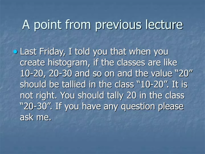
1. A point from previous lecture • Last Friday, I told you that when you create histogram, if the classes are like 10-20, 20-30 and so on and the value “20” should be tallied in the class “10-20”. It is not right. You should tally 20 in the class “20-30”. If you have any question please ask me.

2. Statistical Measures • Although the frequency distribution arranges the raw data into a meaningful pattern, that summary cannot by itself answer many important statistical questions. • For example, an industrial engineer wishing to select the faster of two production methods might obtain sample completion times from pilot runs and then try to reach a decision comparing the two resulting sample frequency distributions.

3. Statistical Measures • The faster procedure ought to be more clearly indicated by the “average “ completion times under the two production methods. • Averages are one class of statistical measures. • These quantities (statistical measures) express various properties of the statistical data.

4. Statistical Measures • First kind of measures in this discussion is Measures of Location • There are two types of location measures. • One group expresses central tendency • The other group measures variability or dispersion.

5. Statistics and Parameter • Summary data measures fall into two major groupings, depending on whether the observations they describe are a population or a sample.

6. Population Parameter • When the data constitute a population, each summary measure is referred to as a population parameter. • But, ordinarily not all possible population observations are made.

7. Sample Statistic • A measure that summarizes sample data is called a sample statistic. • It is the statistic that is computed from those observations actually made. • Important population parameters have counterpart sample statistics that measure the same characteristic.

8. NUMERICAL DESCRIPTIVE MEASURES • Numerical descriptive measures are numbers computed from data set to help us create a mental image of its relative frequency histogram. • Measures of Central Location • Mean, median, mode • Relative Standing • Percentile, box plots • Measures of Variability • Range, • variance, • standard deviation, • Measures of Association • Covariance, coefficient of correlation

9. MEASURES OF CENTRAL LOCATIONMEAN • The arithmetic mean is the most commonly used and best understood measure of central tendency. • Mean is defined as follows: Sum of the measurements Mean = Number of measurements • In the following, sample mean and population means are discussed separately. • Note the difference of notation - sample mean is denote by and the population mean is denoted by . The number of values in a sample is denoted by n and the number of values in the population is denoted by N.

10. Mean of Data Set Data Set is Data Set is Sample Population Sample Population Mean Mean MEASURES OF CENTRAL LOCATIONMEAN

11. MEASURES OF CENTRAL LOCATIONSAMPLE MEAN • The sample mean is the sum of all the sample values divided by the number of sample values: • where stands for the sample mean • n is the total number of values in the sample • is the value of the i- th observation. • represents a summation

12. MEASURES OF CENTRAL LOCATIONSAMPLE MEAN • A sample of five executives received the following amounts of bonus last year: $14,000, $15,000, $17,000, $16,000, and $15,000. Find the average bonus for these five executives. • Since these values represent a sample size of 5, the sample mean is (14,000 + 15,000 +17,000 + 16,000 +15,000)/5 = $15,400.

13. MEASURES OF CENTRAL LOCATIONPOPULATION MEAN • The population mean is the sum of all the population values divided by the number of population values: • Where  stands for the population mean • N is the total number of values in the population • is the value of the i-th observation. • represents a summation

14. MEASURES OF CENTRAL LOCATIONPOPULATION MEAN • The Keller family owns four cars. The following is the mileage attained by each car: 56,000, 23,000, 42,000, and 73,000. Find the average miles covered by each car. • The mean is (56,000 + 23,000 + 42,000 + 73,000)/4 = 48,500

15. MEASURES OF CENTRAL LOCATIONPROPERTIES OF MEAN • Data possessing an interval scale or a ratio scale, usually have a mean. • All the values are included in computing the mean. • A set of data has a unique mean. • The arithmetic mean is the only measure of central tendency where the sum of the deviations of each value from the mean is zero.

16. MEASURES OF CENTRAL LOCATIONPROPERTIES OF MEAN • Consider the set of values: 3, 8, and 4. The mean is 5. Illustrating the last property, (3-5) + (8-5) + (4-5) = -2 +3 -1 = 0. In other words,

17. MEASURES OF CENTRAL LOCATIONMEDIAN • Median: The midpoint of the values after they have been ordered from the smallest to the largest, or the largest to the smallest. There are as many values above the median as below it in the data array. • For an even set of numbers, the median will be the arithmetic average of the two middle numbers. • The median is the most appropriate measure of central location to use when the data under consideration are ranked data, rather than quantitative data. For example, if 13 universities are ranked according to the reputation, university 7 is the one of median reputation.

18. MEASURES OF CENTRAL LOCATIONMEDIAN • Compute the median for the following data. • The age of a sample of five college students is: 21, 25, 19, 20, and 22. • Arranging the data in ascending order gives: 19, 20, 21, 22, 25. Thus the median is 21. • The height of four basketball players, in inches, is 76, 73, 80, and 75. • Arranging the data in ascending order gives: 73, 75, 76, 80. Thus the median is 75.5

19. MEASURES OF CENTRAL LOCATIONMODE • The mode is the value of the observation that appears most frequently. • The mode is most useful when an important aspect of describing the data involves determining the number of times each value occurs. If the data are qualitative (e.g., number of graduate in various disciplines accounting,finance, etc.) then, mode is useful (e.g., a modal class is accounting). • EXAMPLE 6: The exam scores for ten students are: 81, 93, 84, 75, 68, 87, 81, 75, 81, 87. Since the score of 81 occurs the most, the modal score is 81.

20. MEASURES OF CENTRAL LOCATIONMEAN, MEDIAN, MODE • Mean: affected by unusually large/small data, may be used if the data are quantitative (ratio or interval scale). • Median: most appropriate if the data are ranked (ordinal scale) • Mode: most appropriate if the data are qualitative (nominal scale) • Appropriate measures if the data is • quantitative: mean, median, mode • ranked: median, mode • qualitative: mode

21. MEASURES OF CENTRAL LOCATION RELATIVE VALUES OF MEAN, MEDIAN, MODE Mode<Median<Mean If distribution is positively skewed Mode=Median=Mean If distribution is symmetric Mean<Median<Mode if distribution is negatively skewed

22. RELATIVE STANDING PERCENTILES • Percentiles divide the distribution into 100 groups. • The p-th percentile is defined to be that numerical value such that at most p% of the values are smaller than that value and at most (100 – p)% are larger than that value in an ordered data set. • For example, if the 78th percentile of GMAT scores is 600, then at most 78% scores are below 600 and at most 22% scores are above 600 (actually, this is also true that at least 22% are 600 or above). • Percentile gives you an idea about your relative standing in a group. • Two questions: • Find percentile of a given value • Find value of a given percentile

23. number of values below X + 0.5  Percentile  100% total number of values RELATIVE STANDING: PERCENTILESFIND PERCENTILE OF A GIVEN VALUE • The percentile corresponding to a given value (X) is computed by using the formula:

24. RELATIVE STANDING: PERCENTILES FIND PERCENTILE OF A GIVEN VALUE • A teacher gives a 20-point test to 10 students. • Scores are as follows: 18, 15, 12, 6, 8, 2, 3, 5, 20, 10. • Find the percentile rank of the score of 12. • Ordered set of scores: 2, 3, 5, 6, 8, 10, 12, 15, 18, 20. • There are 6 values below 12: 2, 3, 5, 6, 8, 10 • Percentile = [(6 + 0.5)/10](100%) = 65th percentile. Student did better than 65% of the class.

25. RELATIVE STANDING: PERCENTILES FIND VALUE OF A GIVEN PERCENTILE • Procedure: Let p be the percentile and n the sample size. • Step 1: Arrange the data in the ascending order. • Step 2: Compute c = (np)/100. • Step 3: If c is not a whole number, round up to the next whole number. If c is a whole number, use the value halfway between c and c+1. • Step 4: The c-th value of the required percentile.

26. RELATIVE STANDING: PERCENTILES FIND VALUE OF A GIVEN PERCENTILE • Example: Consider data set 2, 3, 5, 6, 8, 10, 12, 15, 18, 20. • Note: the data set is already ordered. • Find the value of the 25th percentile • n = 10, p = 25, so c = (1025)/100 = 2.5. Hence round up to c = 3. Thus, the value of the 25th percentile is the 3rd value X = 5. • Find the value of the 80th percentile • n = 10, p = 80, so c = (1080)/100 = 8. Thus the value of the 80th percentile is the average of the 8th and 9th values. Thus, the 80th percentile for the data set is (15 + 18)/2 = 16.5.

27. RELATIVE STANDING: PERCENTILES DECILES AND QUARTILES • Deciles divide the data set into 10 groups. • Deciles are denoted by D1, D2, …, D9 with the corresponding percentiles being P10, P20, …, P90 • Quartiles divide the data set into 4 groups. • Quartiles are denoted by Q1, Q2, and Q3 with the corresponding percentiles being P25, P50, and P75. • The median is the same as P50 or Q2.

28. RELATIVE STANDING: PERCENTILES INTERQUARTILE RANGE AND OUTLIERS • An outlier is an extremely high or an extremely low data value when compared with the rest of the data values. • The Interquartile Range, IQR = Q3 – Q1. • To determine whether a data value can be considered as an outlier: • Step 1: Compute Q1 and Q3. • Step 2: Find the IQR = Q3 – Q1. • Step 3: Compute (1.5)(IQR). • Step 4: Compute Q1 – (1.5)(IQR) and Q3 + (1.5)(IQR).

29. RELATIVE STANDING: PERCENTILES INTERQUARTILE RANGE AND OUTLIERS • To determine whether a data value can be considered as an outlier: • Step 5: Compare the data value (say X) with Q1–(1.5)(IQR) and Q3 + (1.5)(IQR). • If X < Q1 – (1.5)(IQR) or if X > Q3 + (1.5)(IQR), then X is considered an outlier.

30. RELATIVE STANDING: PERCENTILES INTERQUARTILE RANGE AND OUTLIERS • Given the data set 5, 6, 12, 13, 15, 18, 22, 50, can the value of 50 be considered as an outlier? • Q1 = 9, Q3 = 20, IQR = 11. Verify. • (1.5)(IQR) = (1.5)(11) = 16.5. • 9 – 16.5 = – 7.5 and 20 + 16.5 = 36.5. • The value of 50 is outside the range – 7.5 to 36.5, hence 50 is an outlier.

31. RELATIVE STANDINGBOX PLOTS • When the data set contains a small number of values, a box plot is used to graphically represent the data set. These plots involve five values: • the minimum value (S) • the lower quartile (Q1) • the median (Q2) • the upper quartile (Q3) • and the maximum value (L)

32. RELATIVE STANDING: BOX PLOTSEXAMPLE • Example: Construct a box plot with the following data which shows the assets of the 15 largest North American banks, rounded off to the nearest hundred million dollars: 111, 135, 217, 108, 51 , 98, 65, 85, 75, 75, 93, 64, 57, 56, 98

33. RELATIVE STANDING: BOX PLOTSRANKING AND SUMMARIZING

35. RELATIVE STANDING: BOX PLOTSINTERPRETATION • If the median is near the center of the box, the distribution is approximately symmetric. • If the median falls to the left of the center of the box, the distribution is positively skewed. • If the median falls to the right of the center of the box, the distribution is negatively skewed. • If the lines are about the same length, the distribution is approximately symmetric. • If the line segment to the right of the box is larger than the one to the left, the distribution is positively skewed. • If the line segment to the left of the box is larger than the one to the right, the distribution is negatively skewed.