Download
1 / 43
430 likes | 621 Views
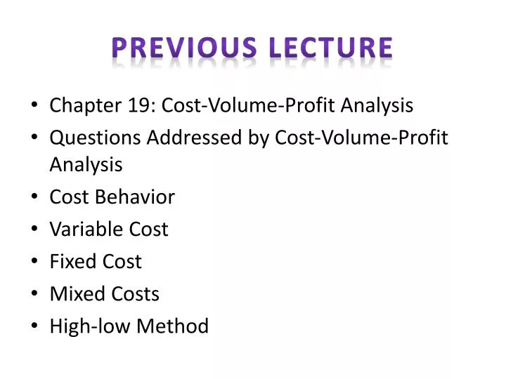
Previous Lecture. Chapter 19: Cost-Volume-Profit Analysis Questions Addressed by Cost-Volume-Profit Analysis Cost Behavior Variable Cost Fixed Cost Mixed Costs High-low Method. Previous Lecture. Stair-Step Costs Curvilinear Costs Cost Behavior Summary Cost-Volume-Profit Relationships

E N D
Previous Lecture • Chapter 19: Cost-Volume-Profit Analysis • Questions Addressed by Cost-Volume-Profit Analysis • Cost Behavior • Variable Cost • Fixed Cost • Mixed Costs • High-low Method
Previous Lecture • Stair-Step Costs • Curvilinear Costs • Cost Behavior Summary • Cost-Volume-Profit Relationships • Contribution Margin Income Statement • Contribution Margin Ratio • Cost-Volume-Profit (CVP) Analysis • Computing Break-Even Point
Previous Lecture • Formula for Computing Break-Even Sales in Units & In Dollar • Preparing a CVP Graph • Computing Sales Needed to Achieve Target Operating Income • What is our Margin of Safety? • What Change in Operating Income Do We Anticipate?
Sales Mix Considerations Chapter19
Products A B Sales $ 90 $140 Variable costs 70 95 Contribution margin $ 20 $ 45 Sales mix 80% 20% Cascade Company sold 8,000 units of Product A and 2,000 units of Product B during the past year. Cascade Company’s fixed costs are $200,000. Other relevant data are as follows:
$25 Sales Mix Considerations Products A B Sales $ 90 $140 Variable costs 70 95 Contribution margin $ 20 $ 45 Sales mix 80% 20% Product contribution margin $16 $ 9 Fixed costs, $200,000
$200,000 $25 $25 Sales Mix Considerations Products A B Product contribution margin $16 $ 9 Break-even sales units Fixed costs, $200,000
Break-even sales units $200,000 $25 $25 Sales Mix Considerations Products A B Product contribution margin $16 $ 9 = 8,000 units Fixed costs, $200,000
$25 Sales Mix Considerations Products A B Product contribution margin $16 $ 9 A:8,000 units x Sales Mix (80%) = 6,400 B:8,000 units x Sales Mix (20%) = 1,600
Product A Product B Total Sales: 6,400 units x $90 $576,000 $576,000 1,600 units x $140 $224,000 224,000 Total sales $576,000$224,000$800,000 Variable costs: 6,400 x $70 $448,000 $448,000 1,600 x $95 $152,000 152,000 Total variable costs $448,000$152,000$600,000 Contribution margin $128,000 $ 72,000 $200,000 Fixed costs 200,000 Income from operations $ 0 Break-even point PROOF
$250,000 – $200,000 $250,000 Margin of Safety = Sales – Sales at break-even point Sales Margin of Safety = Margin of Safety = 20% The margin of safety indicates the possible decrease in sales that may occur before an operating loss results.
Both companies have the same contribution margin. Contribution margin Income from operations Operating Leverage Jones Inc. Wilson Inc. Sales $400,000 $400,000 Variable costs 300,000 300,000 Contribution margin $100,000 $100,000 Fixed costs 80,000 50,000 Income from operations $ 20,000 $ 50,000 Contribution margin ??
5.0 Operating Leverage Jones Inc. Wilson Inc. Sales $400,000 $400,000 Variable costs 300,000 300,000 Contribution margin $100,000 $100,000 Fixed costs 80,000 50,000 Income from operations $ 20,000 $ 50,000 Contribution margin ? Contribution margin Income from operations $100,000 Jones Inc.: = 5.0 $20,000
$100,000 Jones Inc. $20,000 Operating Leverage Jones Inc. Wilson Inc. Sales $400,000 $400,000 Variable costs 300,000 300,000 Contribution margin $100,000 $100,000 Fixed costs 80,000 50,000 Income from operations $ 20,000 $ 50,000 Contribution margin 5.0? Contribution margin Income from operations = 5.0
Capital intensive? Labor intensive? Operating Leverage Jones Inc. Wilson Inc. Sales $400,000 $400,000 Variable costs 300,000 300,000 Contribution margin $100,000 $100,000 Fixed costs 80,000 50,000 Income from operations $ 20,000 $ 50,000 Contribution margin 5.0 2.0 Contribution margin Income from operations $100,000 = 2.0 Wilson Inc.: $50,000
Assumptions of Cost-Volume-Profit Analysis The reliability of cost-volume-profit analysis depends upon several assumptions. 1. Total sales and total costs can be represented by straight lines. 2. Within the relevant rangeof operating activity, the efficiency of operations does not change. 3. Costs can be accurately divided into fixedand variablecomponents. 4. The sales mix is constant. 5. There is no change in the inventory quantities during the period.
Consider the following information developed by the accountant at CyclCo, a bicycle retailer: Business Applications of CVP
Should CyclCo spend $12,000 on advertising to increase sales by 10 percent? Business Applications of CVP
$80K + $12K Business Applications of CVP Should CyclCo spend $12,000 on advertising to increase sales by 10 percent? 550 × $500 550 × $300 No, income is decreased.
Business Applications of CVP Now, in combination with the advertising, CyclCo is considering a 10 percent price reduction that willincrease sales by 25 percent. What is the income effect?
$80K + $12K Business Applications of CVP Now, in combination with the advertising, CyclCo is considering a 10 percent price reduction that willincrease sales by 25 percent. What is the income effect? 1.25 × 500 625 × $450 625 × $300 Income is decreased even more.
Business Applications of CVP Now, in combination with advertising and a price cut, CyclCowill replace $50,000 in sales salaries with a $25 per bike commission, increasing sales by 50 percent above the original 500 bikes. What is the effect on income?
$92K - $50K Business Applications of CVP Now, in combination with advertising and a price cut, CyclCowill replace $50,000 in sales salaries with a $25 per bike commission, increasing sales by 50 percent above the original 500 bikes. What is the effect on income? 1.5 × 500 750 × $450 750 × $325 The combination of advertising, a price cut,and change in compensation increases income.
Different products with different contribution margins. • Determining semivariablecost elements. • Complying with theassumptions of CVP analysis. Additional Considerations in CVP
Sales mix is the relative combination in whicha company’s different products are sold. Different products have different selling prices, costs, and contribution margins. If CyclCo sells bikes and carts, howwill we deal with break-even analysis? CVP Analysis When a Company Sells Many Products
CyclCo provides us with the following information: CVP Analysis When a Company Sells Many Products
The overall contribution margin ratio is: CVP Analysis When a Company Sells Many Products $265,000 $550,000 = 48% (rounded)
Break-even in sales dollars is: CVP Analysis When a Company Sells Many Products $170,000 .48 = $354,167 (rounded)
OwlCo recorded the following production activity and maintenance costs for two months: Using these two levels of activity, compute: the variable cost per unit. the total fixed cost. total cost formula. The High-Low Method
The High-Low Method $3,600 4,000 in costin units • Unit variable cost = = = $0.90 per unit
The High-Low Method $3,600 4,000 in costin units • Unit variable cost = = = $0.90 per unit • Fixed cost = Total cost – Total variable cost
The High-Low Method $3,600 4,000 in costin units • Unit variable cost = = = $0.90 per unit • Fixed cost = Total cost – Total variable cost • Fixed cost = $9,700 – ($0.90 per unit × 9,000 units) • Fixed cost = $9,700 – $8,100 = $1,600
The High-Low Method $3,600 4,000 in costin units • Unit variable cost = = = $0.90 per unit • Fixed cost = Total cost – Total variable cost • Fixed cost = $9,700 – ($0.90 per unit × 9,000 units) • Fixed cost = $9,700 – $8,100 = $1,600 • Total cost = $1,600 + $.90 per unit
If sales commissions are $10,000 when 80,000 units are sold and $14,000 when 120,000 units are sold, what is the variable portion of sales commission per unit sold? a. $.08 per unit b. $.10 per unit c. $.12 per unit d. $.125 per unit The High-Low MethodQuestion 1
If sales commissions are $10,000 when 80,000 units are sold and $14,000 when 120,000 units are sold, what is the variable portion of sales commission per unit sold? a. $.08 per unit b. $.10 per unit c. $.12 per unit d. $.125 per unit The High-Low MethodQuestion 1 $4,000 ÷ 40,000 units = $.10 per unit
If sales commissions are $10,000 when 80,000 units are sold and $14,000 when 120,000 units are sold, what is the fixed portion of the sales commission? a. $ 2,000 b. $ 4,000 c. $10,000 d. $12,000 The High-Low MethodQuestion 2
The High-Low MethodQuestion 2 If sales commissions are $10,000 when 80,000 units are sold and $14,000 when 120,000 units are sold, what is thefixedportion of the sales commission? a. $ 2,000 b. $ 4,000 c. $10,000 d. $12,000
A limited range of activity, called therelevant range, where CVP relationships are linear. Unit selling price remains constant. Unit variable costs remain constant. Total fixed costs remain constant. Sales mix remains constant. Production = sales (no inventory changes). Assumptions Underlying CVP Analysis