Download
1 / 36
360 likes | 704 Views
Indexing Spatial Data (Parts of Chapter 25+R-tree paper). Spatial and Geographic Databases. Spatial databases store information related to spatial locations, and support efficient storage, indexing and querying of spatial data.

E N D
Spatial and Geographic Databases • Spatial databases store information related to spatial locations, and support efficient storage, indexing and querying of spatial data. • Special purpose index structures are important for accessing spatial data, and for processing spatial queries. • Computer Aided Design (CAD) databases store design information about how objects are constructed E.g.: designs of buildings, aircraft, layouts of integrated-circuits • Geographic databases store geographic information (e.g., maps): often called geographic information systems or GIS.
Spatial/Geographic Data • Raster data consist of bit maps or pixel maps, in two or more dimensions. • Example 2-D raster image: satellite image of cloud cover, where each pixel stores the cloud visibility in a particular area. • Additional dimensions might include the temperature at different altitudes at different regions, or measurements taken at different points in time. • Design databases generally do not store raster data.
Spatial/Geographic Data (Cont.) • Vector data are constructed from basic geometric objects: points, line segments, triangles, and other polygons in two dimensions, and cylinders, speheres, cuboids, and other polyhedrons in three dimensions. • Vector format often used to represent map data. • Roads can be considered as two-dimensional and represented by lines and curves. • Some features, such as rivers, may be represented either as complex curves or as complex polygons, depending on whether their width is relevant. • Features such as regions and lakes can be depicted as polygons.
Applications of Geographic Data • Examples of geographic data • map data for vehicle navigation • distribution network information for power, telephones, water supply, and sewage • Vehicle navigation systems store information about roads and services for the use of drivers: • Spatial data: e.g, road/restaurant/gas-station coordinates • Non-spatial data: e.g., one-way streets, speed limits, traffic congestion • Global Positioning System (GPS) unit - utilizes information broadcast from GPS satellites to find the current location of user with an accuracy of tens of meters. • increasingly used in vehicle navigation systems as well as utility maintenance applications.
Representation of Vector Information • Various geometric constructs can be represented in a database in a normalized fashion. • Represent a line segment by the coordinates of its endpoints. • Approximate a curve by partitioning it into a sequence of segments • Create a list of vertices in order, or • Represent each segment as a separate tuple that also carries with it the identifier of the curve (2D features such as roads). • Closed polygons • List of vertices in order, starting vertex is the same as the ending vertex, or • Represent boundary edges as separate tuples, with each containing identifier of the polygon, or • Use triangulation — divide polygon into triangles • Note the polygon identifier with each of its triangles.
Representation of Vector Data (Cont.) • Representation of points and line segment in 3-D similar to 2-D, except that points have an extra z component • Represent arbitrary polyhedra by dividing them into tetrahedrons, like triangulating polygons.
Spatial Queries • Nearness queries request objects that lie near a specified location. • Nearest neighbor queries, given a point or an object, find the nearest object that satisfies given conditions. • Region queries deal with spatial regions. e.g., ask for objects that lie partially or fully inside a specified region. • Queries that compute intersections or unions of regions. • Spatial join of two spatial relations with the location playing the role of join attribute.
Spatial Queries (Cont.) • Spatial data is typically queried using a graphical query language; results are also displayed in a graphical manner. • Graphical interface constitutes the front-end • Extensions of SQL with abstract data types, such as lines, polygons and bit maps, have been proposed to interface with back-end. • allows relational databases to store and retrieve spatial information • Queries can use spatial conditions (e.g. contains or overlaps). • queries can mix spatial and nonspatial conditions
Indexing of Spatial Data • k-d tree - early structure used for indexing in multiple dimensions. • Each level of a k-d tree partitions the space into two. • choose one dimension for partitioning at the root level of the tree. • choose another dimensions for partitioning in nodes at the next level and so on, cycling through the dimensions. • In each node, approximately half of the points stored in the sub-tree fall on one side and half on the other. • Partitioning stops when a node has less than a given maximum number of points. • The k-d-B tree extends the k-d tree to allow multiple child nodes for each internal node; well-suited for secondary storage.
Division of Space by a k-d Tree • Each line in the figure (other than the outside box) corresponds to a node in the k-d tree • the maximum number of points in a leaf node has been set to 1. • The numbering of the lines in the figure indicates the level of the tree at which the corresponding node appears.
Division of Space by Quadtrees Quadtrees • Each node of a quadtree is associated with a rectangular region of space; the top node is associated with the entire target space. • Each non-leaf node divides its region into four equal sized quadrants • correspondingly each such node has four child nodes corresponding to the four quadrants and so on • Leaf nodes have between zero and some fixed maximum number of points (set to 1 in example).
Quadtrees (Cont.) • PR quadtree: stores points; space is divided based on regions, rather than on the actual set of points stored. • Region quadtrees store array (raster) information. • A node is a leaf node is all the array values in the region that it covers are the same. Otherwise, it is subdivided further into four children of equal area, and is therefore an internal node. • Each node corresponds to a sub-array of values. • The sub-arrays corresponding to leaves either contain just a single array element, or have multiple array elements, all of which have the same value. • Extensions of k-d trees and PR quadtrees have been proposed to index line segments and polygons • Require splitting segments/polygons into pieces at partitioning boundaries • Same segment/polygon may be represented at several leaf nodes
R-Trees • R-trees are a N-dimensional extension of B+-trees, useful for indexing sets of rectangles and other polygons. • Supported in many modern database systems • Basic idea: generalize the notion of a one-dimensional interval associated with each B+ -tree node to an N-dimensional interval, that is, an N-dimensional rectangle. • Will consider only the two-dimensional case (N = 2) • generalization for N > 2 is straightforward
Bounding Rectangle Suppose we have a cluster of points in 2-D space... We can build a “box” around points. The smallest box (which is axis parallel) that contains all the points is called a Minimum Bounding Rectangle (MBR) also known as minimum bounding box MBR = {(L.x,L.y)(U.x,U.y)} Note that we only need two points to describe an MBR, we typically use lower left, and upper right.
Clustering Points We can group clusters of datapoints into MBRs Can also handle line-segments, rectangles, polygons, in addition to points R1 R4 R2 R5 R3 R6 R9 R7 R8 We can further recursively group MBRs into larger MBRs….
R-Tree Structure Nested MBRs are organized as a tree R10 R11 R12 R10 R11 R12 R1 R2 R3 R4 R5 R6 R7 R8 R9 Data nodes containing points
R Trees (Cont.) • A rectangular bounding box (a.k.a. MBR) is associated with each tree node. • Bounding box of a leaf node is a minimum sized rectangle that contains all the rectangles/polygons associated with the leaf node. • The bounding box associated with a non-leaf node contains the bounding box associated with all its children. • Bounding box of a node serves as its key in its parent node (if any) • Bounding boxes of children of a node are allowed to overlap • A polygon is stored only in one node, and the bounding box of the node must contain the polygon • The storage efficiency or R-trees is better than that of k-d trees or quadtrees since a polygon is stored only once
Example R-Tree • A set of rectangles (solid line) and the bounding boxes (dashed line) of the nodes of an R-tree for the rectangles. The R-tree is shown on the right.
Search in R-Trees • To find data items (rectangles/polygons) intersecting (overlaps) a given query point/region, do the following, starting from the root node: • If the node is a leaf node, output the data items whose keys intersect the given query point/region. • Else, for each child of the current node whose bounding box overlaps the query point/region, recursively search the child • Can be very inefficient in worst case since multiple paths may need to be searched • but works acceptably in practice. • Simple extensions of search procedure to handle • predicates contained-in and contains • Find data items nearest to a given point • Find data items within a given distance of a given point
Nearest Neighbor Search Given an MBR, we can compute lower bounds on nearest object Once we know there IS an item within some distance d, we can prune away all items/MBRs at distance > d Even if we haven’t actually found the nearest item yet Similar technique possible for k-d trees and quadtrees as well R10 R11 R10 R11 R12 R1 R2 R3 R4 R5 R6 R7 R8 R9 R12 Data nodes containing points Q
MBR: Distance Calculation The formula for the distance between a point and the closest possible point within an MBR MBR = {(L.x,L.y)(U.x,U.y)} Q = (x,y) MINDIST(Q,MBR) if L.x < x < U.x and L.y < y < U.y then 0 elseif L.x < x < U.x then min( abs(L.y -y) , abs(U.y -y) ) elseif ….
MBR: Distance Example Two examples of MINDIST(point, MBR), calculations… MINDIST(point, MBR) = 5 MINDIST(point, MBR) = 0
MBR: Distance Bounds • Distance bounds on bounding boxes • Suppose we have a query point Q and one known point R • Could any of the points in the MBR be closer to Q than R is? R = (1,7) Q = (3,5) MBR = {(6,1),(8,4)}
Insertion in R-Trees To insert a data item E: Find a leaf to store it, and add it to the leaf To find leaf, starting from root, at each step: follow a child (if any) whose bounding box contains bounding box of data item, else child whose bounding box needs least enlargement to contain data item E Handle overflows by splits (as in B+ -trees) Split procedure is different though (see below) Adjust bounding boxes starting from the leaf upwards Split procedure: Goal: divide entries of an overfull node into two sets such that the bounding boxes have minimum total area This is a heuristic. Alternatives like minimum overlap are possible Finding the “best” split is expensive, use heuristics instead See next slide
Splitting a Node • (Heuristic) goal: find split whose total area is maximized. • Minimizes chances that the nodes will be searched • Finding best split is expensive (not exponential time, but costly)
Splitting an R-Tree Node Quadratic split divides the entries in a node into two new nodes as follows Find pair of entries with “maximum separation” that is, the pair such that the bounding box of the two would have the maximum wasted space (area of bounding box – sum of areas of two entries) Place these entries in two new nodes Repeatedly find the entry with “maximum preference” for one of the two new nodes, and assign the entry to that node Preference of an entry to a node is the increase in area of bounding box if the entry is added to the other node Stop when half the entries have been added to one node Then assign remaining entries to the other node
Linear Split • Cheaper linear split heuristic works in time linear in number of entries, • Cheaper but generates slightly worse splits. • Idea: pick extreme elements by choosing dimension with maximum (normalized) separation between rectangle with highest low side and lowest high side • Normalize each dimension by scaling to 1 • Choose entries in any order • For each one assign to side that results in least area increase • Until one side has > ½ entries, then assign all to other side
Deleting in R-Trees Deletion of an entry in an R-tree can be done much like a B+-tree deletion. In case of underfull node, borrow entries from a sibling if possible, else merging sibling nodes Alternative approach removes all entries from the underfull node, deletes the node, then reinserts all entries Goal: improve locality of R-tree by reinserting nodes Described in detail in paper in Algorithm CondenseTree
Design Databases • Represent design components as objects (generally geometric objects); the connections between the objects indicate how the design is structured. • Simple two-dimensional objects: points, lines, triangles, rectangles, polygons. • Complex two-dimensional objects: formed from simple objects via union, intersection, and difference operations. • Complex three-dimensional objects: formed from simpler objects such as spheres, cylinders, and cuboids, by union, intersection, and difference operations. • Wireframe models represent three-dimensional surfaces as a set of simpler objects.
Representation of Geometric Constructs (a) Difference of cylinders (b) Union of cylinders • Design databases also store non-spatial information about objects (e.g., construction material, color, etc.) • Spatial integrity constraints are important. • E.g., pipes should not intersect, wires should not be too close to each other, etc.
R10 {(1,0),(7,9)} R1 R2 R3 {(1,3),(5,4)} {(2,0),(7,9)} {(1,1),(7,8)} R12 (5,1) 32 (1,4) 45 (5,6) 27 (7,8) 73 (3,4) 77 (1,3) 88 (2,3) 22 (5,4) 13 (2,2) 47 (3,0) 86 (7,9) 52 At the leaf nodes we have the location, and a pointer to the record in question. At the internal nodes, we just have MBR information. Data nodes