Download
1 / 56
570 likes | 1.03k Views
Morphing. Morphing vs deformation Image morphing Polygon-morphing Triangle-mesh morphing Morphing between animation frames (slow-motion) Mapping textures and parametric correspondence. Updated September 14, 2014. Morphing vs deformation. Deformation

E N D
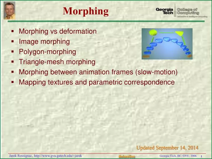
Morphing • Morphing vs deformation • Image morphing • Polygon-morphing • Triangle-mesh morphing • Morphing between animation frames (slow-motion) • Mapping textures and parametric correspondence Updated September 14, 2014
Morphing vs deformation • Deformation • Input: Initial shape A + warp (designed or simulated) • Result of computation: Final shape • Animation: Apply the warp progressively (bundle its parameters) • Morphing • Input: Initial and final shapes A and B • Result of computation: Warp • Animation: Apply the warp progressively (bundle its parameters) • Both can be combined
Cohen-Or et al. Image morph: warp and blend
Image morph by fitting a surface in 3D Fit surface in 3D Stack of 2D slices Simplify surface • “Surface simplification and Edgebreaker compression for 2D Cel Animations”, Kwatra & Rossignac, Shape Modeling International, 2001. Simplified animation Cross-section
3D applications migrated from slices to 3D Early 3D GIS, Medical, and M-CAD systems were based on stacks of cross-sections They migrated to continuous 3D models, so that they could better support: simplification Boolean operations compression rendering interferencedetection segmentation editing analysis
Need a similar migration for animations (x,y,z,t) • Represent & slice a hyper-surface in 4D • Voxels or Tetrahedra in 4D: • (x,y,z,t)+connectivity? • Fast slice of hypercubes or tetrahedra • Addressed by Jack Snoeyink’s CARGO project • Generate interpolating 4D models • 3D morph, fitting implicit hyper-surface • Use 4D model to buildtemporally coherent segmentationsof the evolving shape into features? • Use 4D model to buildtemporally coherent parameterizationsof the evolving features? t ?
A 4D model of the behavior of 3D shapes Many animation and simulation packages represent behavior as a series of independent 3D frames Yet, a continuous model is better suited for supporting slow-motion, geometric and topological analysis, and coherent segmentation, texturing and visualization Geometry: x,y,z ? Shape M(t2) is the cross-section of a 4D model by the plane t= t2 t0 t1 t2 t3 t t4 Time: t
How to generate a continuous 4D model? • Design by manipulating control points of B-spline S(u,v,t) • Fit a hyper-surface to constraints • As we did by fitting a surface to a stack of contours • Piecewise linear or polynomial morphs between 3D frames
Minkowski sum Region swept by B when its origin wanders all over A If B is small, then the result is similar to A (and vice versa) Hence, we combine scaling with : (1–t)AtBWhen t=0, we obtain A. When t=1, we obtain B The result is independent of the choice of origin
B D A C E 2D morph • Each edge morphs to at least one vertex of the other shape • Morph(A,B,D,t) produces an edge between (1–t)A+tD and (1–t)B+tD • Replace t by 1–t when morphing the edges of the other curve
B D A C E Minkowski morph in 2D for (int i=0; i<nP; i++) { // for all vertices A in P, for (int j=0; j<nQ; j++) { //for all vertices D in Q pt A = P[i]; pt B = P[in(i)]; pt C = Q[jp(j)]; pt D = Q[j]; pt E = Q[jn(j)]; if ( (dot(A.vecTo(B).left(),D.vecTo(C)) > 0) // if AB.left * DC <0 && (dot(C.vecTo(D).left(),C.vecTo(E)) > 0) // skip concave vertices && (dot(A.vecTo(B).left(),D.vecTo(E)) > 0) ) // and if AB.left * DE <0 morph(A,B,D,t); // morph edge(A,B) of P with vertex D of Q }; }; … swap P and Q and redo
Minkowski morph in 2D results Works for some non convex pairs
A+B A B 3D morphing via Minkowski averaging • A+B = {a+b: aA, bB} • Matches boundary points with same normal • M(t)=(1-t)A+tB “Solid-Interpolating Deformations: Construction and Animation of PIPs”, Kaul&Rossignac, C&G’92, 16(1)107-115. • Constant connectivity, linear trajectory • Realtime animation • Vertices move on straight lines • May be extended to more solids and motions along Bezier curves t
FA VB EA The faces of a Minkowski morph Match face-to-vertex or edge-to-edge when each blue tangent has a negative dot product with the red normal Traveling triangle EB Vertices travel along straight lines Traveling parallelogram Need only match convex edges
b1 a1 a1 b1 a2 b2 a2 a3 Algorithm • Establish mappings between pairs: Vertex-triangle, Edge-edge. Triangle-vertex • Build a triangle list, whose vertices are each represented by a reference to a vertex of A and a reference to a vertex of B • During animation, pre-compute (1–t)ai and tbj, then render using + Each vertex of M(t)=(1-t)A+tB linearly interpolates a vertex of A and a vertex of B
Faces of a Minkowski morph • Face-to-vertex (green) • Edge-to-edge (red) • Vertex-to-face (blue)
Minkowski morphs for design • Rounding • Blending • Creating new shapes
Morphing non-convex shapes May produce multiple branches and self-intersections
A+B A B t Bezier morphs with 4 control shapes • A+B = {a+b: aA, bB} • M(t)=(1-t)A+tB M(t)= (1-t)((1-t)((1-t)A+tB)+t((1-t)B+tC))+t((1-t)((1-t)B+tC)+t((1-t)C+tD)) “AGRELs and BIPs: Metamorphosis as a Bezier curve in the space of polyhedra”, Rossignac&Kaul, CGForum’94, 13(3)179-184. • Vertices move on Bezier curves
Combine morph with polyscrew motion • Move coordinate system while performing the morph • Given 2 or more shapes, align them (registration) to define the motion, then compute the Minkowski morph of the aligned shapes
Tangent Ball map & morph • Distance between shapes • Discrepancy measures (Hausdorff, Frechet, Tangent Ball) • Closest Point (CP) and Tangent Ball (TB) map and morph • Relative rounding
Motivation Dimension and tolerancing of machined parts Specify allowable discrepancy in shape Manufacturing inspection and yield control Visualize areas where the process deviates from nominal Bone grafting Ensure that the graft perfectly matches the desired shape Shape Simplification Measure the discrepancy between original and approximation Animation Morph between two similar shapes Rendering Map textures between different shapes Analysis Track/transfer properties between (evolving) (iso) surfaces G. Turk et al.
Ball distance new DBall(P,Q) = Diameter of largest ball that fits in the gap and touches both shapes Good measure if shapes are b-compatible (single point contacts) Takes distance and orientation into account. Can be extended to incompatible shapes
Our “Tangent Ball” b-map • = (iPiQ) (PQ)is the gap between the two shapes • TPQ is the set of disks/balls in that touch both P and Q • BPQ maps SP to SQ for each disk S ofTPQ Definition works in 2D (disks) and 3D (balls) gap Disks ofTPQ
B-map advantages • BPQ is symmetric: BQP(BPQ(p))=p • BPQ is sensitive to the orientation of both shapes
A B B-compatible curves Two curves A and B are b-compatible if H(A,B) < max(LFS(A), LFS(B)) • h < f P and Q are b-compatible h = Hausdorffdistance between A and B. h = smallest r such that ABr and BAr, where Xr is the set of points at distance r or less from X. f = min( mfs(A ) , mfs( B ) ) minimum feature size mfs(X) = largest r such that X=Fr(X) where Fr(X) is the set not reachable by open r-ball not intersecting X • h < f isless constraining than: h < 0.58f P and Q are c-compatible
Comparing compatibility conditions • P and Q are c-compatible when both CPQ and CQPare homeomorphisms • c-compatibility implies b-compatibility • P and Q are b-compatible when BPQ is a homeomorphism not c-compatible b-compatible
!P P iP Good Bad: disconnected Restrictions for b-morphing • P and Q are boundaries (curves in 2D, surfaces in 3D) of regularized regions (area, solid) iP is the finite interior (region) bounded by P !P is the exterior (complement of PiP) • We assume that: • P and Q are connected and manifold • iPiQ is connected • !P!Q is connected
B-morph with circular trajectories • Circular trajectories • Normal incidence on both shapes
Approximating the middle set • Constrained Delaunay triangulation • Join the centers of adjacent triangles (no bifurcation!)
Average travel distance b-morph requires less average travel than either c-morphs when integrated over the median or over both shapes c-morph from P to Q, ||p’q||: 3555 c-morph from Q to P, ||q’p||: 3560 Straight-line b-morph, ||pq||: 3464 Circular b-morph, arc-length: 3492
Fitting surface between cross-sections The b-morph yields an interpolating surface with a smaller surface area and a “nicer” shape Two c-morphs and a b-morph. Which one is the “nicest”?
Discrepancy between b-compatible shapes • Local measure: length of arc from p • Global measure: Integral of arc-length trajectory • Integrate over M, H, or P & Q • L1, L2, L • When h<f: length of longest arc = DHaus(P,Q) = DFre(P,Q)
Distortion Ball morph between linear sections is distortion free and in general is closer to normal (c-morph) flow
b-map computation • Grow tangent ball at p in the gap until it touches Q. m = p +rNP(p) find smallest r such that Dist(m,Q)=r Solve for all elements of Q (points, line segments, arcs, triangles…). Return smallest r>0
Mid-edge to vertex b-morph • E=(A+B)/2 // mid edge point • N=(B–A).left.unit // normal to edge • Find r such that (E+rN–C)2=r2 (CE+rN)2=r2 since V2=VV, distribute over + CE2+r2N2 +2rCEN=r2 sinceN2 =1, subtract r2 on both sides CE2+2rCEN=0 r= –CE2 / (2CEN) C r r N A E B
Lacing PCCs Linear cost algorithm for b-compatible piecewise circular curves • March on both curves • Compute the images of the end-points of current edge • Take the smallst of the two steps Divides the gap into slabs, each bounded by 4 arcs
B-offset reconstruction Express Q as the b-offset of P Represent it by P and the offset field r(p) Reconstruct Q by computing: m=p+rNP(p) N = normal to M at m (from derivatives of r in tangent plane) q=p+2(pmN)N
Exaggeration Barely noticeable discrepancies between b-compatible shapes may be exagerated by scaling the field r
Progressive offset Increasing the scaling of r from 0 to 1 creates a morph that sweeps the gap
B-morph • Each sample travels on its circular arc from p to q
B-morph synchronization • Regular: Constant speed for each trajectory • Computed so that they all start and stop at the same time • Invading: Same speed for all, starting at P • Symmetric: Same speed for all, simultaneously passing H
Non b-compatible shapes Assume now that P and Q are not b-compatibile One of the c-maps can still be a homeomorphism CPQ can be a homeomorphism, while CQP and BPQ are not
Composite b-morph • Compute b-roundings P1 =bRound(P,Q), Q1=bRound(Q,P) • Then recursively: Pi+1=bRound(P,Pi), Qi+1=bRound(Q,Qi+1) • Stop when P=Pi or when CP Pi is a homeomorphism • Note that trajectories are smoothly connected PCCs
Synchronization of composite b-morphs Regular: Each morph has constant speed Invading: All same speed staring at one shape Symmetric: Same speed, synchronized at H