Download

1 / 50
510 likes | 629 Views
Click to see more. Rate of Change And Limits. What is Calculus?. Two Basic Problems of Calculus. ( x , f( x )). . ( x , f( x )). . . ( x , f( x )). 1. Find the slope of the curve y = f ( x ) at the point ( x , f ( x )). Area.

E N D
Click to see more. Rate of Change And Limits What is Calculus?
Two Basic Problems of Calculus (x, f(x)) (x, f(x)) (x, f(x)) 1. Find the slope of the curve y = f (x) at the point (x, f (x))
Area 2. Find the area of the region bounded above by the curve y = f(x), below by the x-axis and by the vertical lines x = a and x = b y = f(x) x a b
From BC (before calculus) We can calculate the slope of a line given two points Calculate the slope of the line between the given point P (.5, .5) and another point on the curve, say Q(.1, .99). The line is called a secant line. .
Slope of Secant line PQ P(0.5, 0.5) Point Q Let x values get closer and closer to .5. Determine f(x) values.
Slope of Secant line PQ As Q gets closer to P, the Slope of the secant line PQ Gets closer and closer to the slope Of the line tangent to the Curve at P.
Slope of a curve at a point Figure 1.4: The tangent line at point P has the same steepness (slope) that the curve has at P. The slope of the curve at a point P is defined to be the slope of the line that is tangent to the curve at point P. In the figure the point is P(0.5, 0.5)
Slope formula In calculus we learn how to calculate the slope at a given point P. The strategy is to take use secant lines with a second point Q. and find the slope of the secant line. Continue by choosing second points Q that are closer and closer to the given point P and see if the difference quotient gets closer to some fixed value. .
Slope Find the slope of y = x2 at the point (1,1) Find the equation of the tangent line. A
Find slope of tangent line on f(x) =x2 at the point (1,1) Approaching x = 1 from the right Slope appears to be getting close to 2.
Find slope of tangent line on f(x) =x2 at the point (1,1) Approaching x = 1 from the left Slope appears to be getting close to 2.
Write the equation of tangent line • As the x value of the second point gets closer and closer to 1, the slope gets closer and closer to 2. We say the limit of the slopes of the secant is 2. This is the slope of the tangent line. • To write the equation of the tangent line use the point-slope formula
Average rate of change (from bc) If f(t) represents the position of an object as a function of time, then the rate of change is the velocity of the object. Find the average velocity if f (t) = 2 + cost on [0, ] 1. Calculate the function value (position) at each endpoint of the interval f() = 2 + cos () = 2 – 1 = 1 f(0) = 2 + cos (0) = 2 + 1 = 3 2. Use the slope formula The average velocity on on [0, ] is
Instantaneous rate of change To calculate the instantaneous rate of change of we could not use the slope formula since we do not have two points. To approximate instantaneous calculate the average rates of change in shorter and shorter intervals to approximate the instantaneous rate of change.
2.2 To understand the instantaneous rate of change (slope) problem and the area problem, you will need to learn about limits
Limits We write this as: The answer can be found graphically, numerically and analytically. What happens to the value of f (x) when the value of x gets closer and closer and closer (but not necessarily equal) to 2?
20 18 16 14 12 10 8 6 4 2 5 4 3 2 2 1 0 1 2 3 4 5 4 GraphicalAnalysis f (x) x What happens to f(x) as x gets closer to 2?
Numerical Analysis Use one sided limits Start to the left of 2 and choose x values getting closer and closer (but not equal) to 2 x 1.5 1.9 1.99 1.999 1.9999 f (x) 9.25 11.41 11.941 11.994001 11.99940001 Could x get closer to 2? Does f(x) appear to get closer to a fixed number?
Numerical Analysis Start to the right of 2 and choose x values getting closer and closer (but not equal ) to 2 x 2.5 2.1 2.01 2.001 2.0001 f (x) 15.3 12.61 12.0601 12.006001 12.00060001 If the limit exists, f(x) must approach the same value from both directions. Does the limit exist? Guess what it is.
Limits that do not exist Figure 1.8: The functions in Example 7. In order for a limit to exist, the function must approach the same value From the left and from the right.
Infinite Limits What happens to the function value as x gets closer and closer to 3 from the right? The function increases without bound so we say There is a vertical asymptote at x = 3.
The line x=a is a Vertical Asymptote if at least one is true. Identify any vertical asymptotes:
(b) (c) Graph of f(x) True or false • x = 2 is in the domain of f
2.3 Functions That Agree at All But One Point If f(x) = g(x) for all x in an open interval except x = c then: Example then Evaluate by direct substitution 2-5 = -3 As x gets closer and closer and closer to 2, the function value gets closer and closer to -3.
= Analytic = Using direct substitution, As x gets closer and closer to 2 (but not equal to 2) f(x) gets closer and closer to 12
1. 2. 3. Basic Limits If b and c are real numbers and is n a positive integer Guess an answer and click to check. Guess an answer and click to check. Guess an answer and click to check. = -2 Ex: = 5 Ex: = 9 Ex:
Properties of Limits Multiplication by a constant b Limit of a sum or difference Limit of a product Limit of a power Limit of a quotient when denominator is not 0.
Using Properties of Limits Properties allow evaluation of limits by direct substitution for many functions. Ex.: As x gets closer and closer to 3, the function value gets closer and closer to 9.
Analytic Techniques Direct substitution • First substitute the value of x being approached into the function f(x). If this is a real number then the limit is that number. • If the function is piecewise defined, you must perform the substitution from both sides of x. The limit exists if both sides yield the same value. If different values are produced, we say the limit does not exist.
Analytic Techniques Rewrite algebraically if direct substitution produces an indeterminate form such as 0/0 • Factor and reduce • Rationalize a numerator or denominator • Simplify a complex fraction When you rewrite you are often producing another function that agrees with the original in all but one point. When this happens the limits at that point are equal.
0 0 Find the indicated limit direct substitution fails Rewrite and cancel = - 5 now use direct sub.
0 0 Find the indicated limit direct substitution fails Rewrite and cancel now use direct sub.
Find the indicated limit 5 calculate one sided limits 7 Since the one-sided limits are not equal, we say the limit does not exist. There will be a jump in the graph at x =2
Determine the limit on y = sin θ/θ as θ approaches 0. Although the function is not defined at θ =0, the limit as θ 0 is 1. Figure 1.24: The graph of f () = (sin )/.
A one-sided limit Figure 1.37: The graph of y = e1/x for x < 0 shows limx0–e1/x = 0. (Example 11)
Limits that are infinite (y increases without bound) An infinite limit will exist as x approaches a finite value when direct substitution produces If an infinite limit occurs at x = c we have a vertical asymptote with the equation x = c.
2.5 Continuity in (a) at x = 0 but not in other graphs. Figure 1.50: The function in (a) is continuous at x = 0; the functions in (b) through ( f ) are not.
Conditions for continuity A function y = f(x) is continuous at x = c if and only if: • The function is defined at x = c • The limit as x approaches c exists • The value of the function and the value of the limit are equal.
Composite Functions Figure 1.53: Composites of continuous functions are continuous. If two functions are continuous at x = c then their composition will be continuous. is continuous for all reals. Example:
Exploring Continuity Are there values of c and m that make the function continuous At x = 1? Find c and m or tell why they do not exist.
s(t) = 8(t3 – 6 t2 +12t) • t s • 0 0 • 56 • 64 • 72 Position of a car at t hours. 1. Draw a graph. 2. Does the car ever stop? 3. What is the average velocity for the following intervals a. [0, 2], b. [.5, 1.5] c. [.9,1.1] 4. Estimate the instantaneous velocity at t = 1
s(t) = 8(t3 – 6 t2 +12t) 2. Appears to stop at t =2. (Velocity= 0) 3. What is the average velocity for [0, 2], [.5, 1.5] [.9,1.1] a) 31 mph b) 26 mph c) 24.08 mph
Find an equation of the tangent line to y = 2x3 – 4 at the point P(2, 12) So, m = 24. Use the point slope form to write the equation
Figure 1.62: The tangent slope is Slope of the tangent line at x= a f (x0 + h) – f (x0) h lim h0 Q(a + h, f (a + h)) f(a+h) – f(a) P(a, f(a)) a + h a
Other form for Slope of secant line of tangent line Let h = x - a Then x = a + h
Find an equation of the tangent line at (3, ½) to At a = 3, m = - 1/8 Using the point-slope formula: